Mapa Genético

workflowr

• Summary
• Checks
• Past versions

Last updated: 2025-03-25

Checks: 7 0

Knit directory: Genomic-prediction-through-machine-learning-and-neural-networks-for-traits-with-epistasis/

This reproducible R Markdown analysis was created with workflowr (version 1.7.1). The Checks tab describes the reproducibility checks that were applied when the results were created. The Past versions tab lists the development history.

---

R Markdown file: up-to-date

Great! Since the R Markdown file has been committed to the Git repository, you know the exact version of the code that produced these results.

Environment: empty

Great job! The global environment was empty. Objects defined in the global environment can affect the analysis in your R Markdown file in unknown ways. For reproduciblity it’s best to always run the code in an empty environment.

Seed: set.seed(20220720)

The command set.seed(20220720) was run prior to running the code in the R Markdown file. Setting a seed ensures that any results that rely on randomness, e.g. subsampling or permutations, are reproducible.

Session information: recorded

Great job! Recording the operating system, R version, and package versions is critical for reproducibility.

Cache: none

Nice! There were no cached chunks for this analysis, so you can be confident that you successfully produced the results during this run.

File paths: relative

Great job! Using relative paths to the files within your workflowr project makes it easier to run your code on other machines.

Repository version: 6961890

Great! You are using Git for version control. Tracking code development and connecting the code version to the results is critical for reproducibility.

The results in this page were generated with repository version 6961890. See the Past versions tab to see a history of the changes made to the R Markdown and HTML files.

Note that you need to be careful to ensure that all relevant files for the analysis have been committed to Git prior to generating the results (you can use wflow_publish or wflow_git_commit). workflowr only checks the R Markdown file, but you know if there are other scripts or data files that it depends on. Below is the status of the Git repository when the results were generated:

Ignored files:
    Ignored:    .Rproj.user/

Note that any generated files, e.g. HTML, png, CSS, etc., are not included in this status report because it is ok for generated content to have uncommitted changes.

---

These are the previous versions of the repository in which changes were made to the R Markdown (analysis/map.Rmd) and HTML (docs/map.html) files. If you’ve configured a remote Git repository (see ?wflow_git_remote), click on the hyperlinks in the table below to view the files as they were in that past version.

File	Version	Author	Date	Message
html	492212b	WevertonGomesCosta	2025-03-24	add map.html
Rmd	9939fd8	WevertonGomesCosta	2025-03-24	add setup knitr::opts_chunk\(set(echo = T, warning = F, message = F)</td> </tr> <tr> <td>Rmd</td> <td><a href="https://github.com/WevertonGomesCosta/Genomic-prediction-through-machine-learning-and-neural-networks-for-traits-with-epistasis/blob/64ac53e09afdb8cd6d5cd4f655fa232c644d2fb3/analysis/map.Rmd" target="_blank">64ac53e</a></td> <td>WevertonGomesCosta</td> <td>2025-03-24</td> <td>add setup knitr::opts_chunk\)set(echo = T, warning = F, message = F)
Rmd	550dccd	WevertonGomesCosta	2025-03-24	add map.rmd

---

Genomic prediction through machine learning and neural networks for traits with epistasis

Creating Genetic Map Chart

Libraries

library(tidyverse)
library(data.table)
library(ggthemes)
library(ggrepel)
library(ggpubr)
library(cowplot)
library(tidytext)

Phenotypic variance and genetic values

pheno <- read.table("data/simulated_data/phenotype.txt")

colnames(pheno) <- str_replace_all(colnames(pheno), "V", "P")

genetic_values <-
  read.table("data/simulated_data/genotypic values.txt")

colnames(genetic_values) <-
  str_replace_all(colnames(genetic_values), "V", "G")

pheno <- pheno %>%
  pivot_longer(1:18) %>%
  mutate(trait = as.numeric(factor(name)))

genetic_values <-  genetic_values %>%
  pivot_longer(1:18) %>%
  mutate(trait = as.numeric(factor(name)))

data <- pheno %>%
  full_join(genetic_values) %>%
  mutate(type = ifelse(name %like% "P", "Phenotype", "Genetic"))

data  %>%
  ggplot(aes(x = as.factor(trait), y = value, fill = type)) +
  geom_boxplot() +
  ylim(0, 120) +
  scale_fill_gdocs() +
  theme_bw() +
  theme(text = element_text(size = 20, face = "bold")) +
  labs(x = "Traits",
       y = "Value",
       fill = "Type")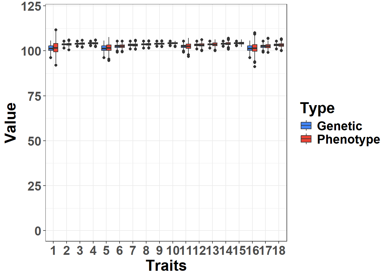

Past versions of unnamed-chunk-2-1.png

Version	Author	Date
492212b	WevertonGomesCosta	2025-03-24

Genetic map

Primeiro vamos definir nossos SNPs de interesse para as variáveis. Essas informações foram pré-definidas e podem ser encontrados no arquivo control_genetic. Vamos carregar o arquivo snpsOfInterest.RData que comtemas infomações dos snps considerados QTLs por variavel.

load("analysis/snpsOfInterest.RData")

Agora vamos definir os nomes das colunas para nosso snpsOfInterest e criar um objeto locus com as informações de ininício e témino de cada grupo de ligação.

locus <-
  data.frame(
    c(
      1,
      401,
      402,
      802,
      803,
      1203,
      1204,
      1604,
      1605,
      2005,
      2006,
      2406,
      2407,
      2807,
      2808,
      3208,
      3209,
      3609,
      3610,
      4010
    )
  )

colnames(locus) <- c("marker")

Para facilitar a visualização criei um gráfico genético das características map_plot. Para isso criei o map com o número de marcadores e tamanho de cada grupo de liagação.

letters <- c("A", "B", "C", "D", "E")

map <-
  data.frame(rbind(
    cbind(seq(1, 401, 1), rep("LG 1", 401), seq(0, 200, 0.5)),
    cbind(seq(402, 802, 1), rep("LG 2", 401), seq(0, 200, 0.5)),
    cbind(seq(803, 1203, 1), rep("LG 3", 401), seq(0, 200, 0.5)),
    cbind(seq(1204, 1604, 1), rep("LG 4", 401), seq(0, 200, 0.5)),
    cbind(seq(1605, 2005, 1), rep("LG 5", 401), seq(0, 200, 0.5)),
    cbind(seq(2006, 2406, 1), rep("LG 6", 401), seq(0, 200, 0.5)),
    cbind(seq(2407, 2807, 1), rep("LG 7", 401), seq(0, 200, 0.5)),
    cbind(seq(2808, 3208, 1), rep("LG 8", 401), seq(0, 200, 0.5)),
    cbind(seq(3209, 3609, 1), rep("LG 9", 401), seq(0, 200, 0.5)),
    cbind(seq(3610, 4010, 1), rep("LG 10", 401), seq(0, 200, 0.5))
  ))

colnames(map) <- c("marker", "LG", "Size")

map <- map %>%
  mutate(
    marker = as.numeric(marker),
    Size = as.numeric(Size),
    LG = factor(
      LG,
      levels = c(
        "LG 1",
        "LG 2",
        "LG 3",
        "LG 4",
        "LG 5",
        "LG 6",
        "LG 7",
        "LG 8",
        "LG 9",
        "LG 10"
      )
    )
  )

Para dividir a figura e mostrar todos os maps genômicos das características, dividi o snpsOfInterest e o map para cada característica e inclui os SNPs de interesse no map para cada característica.

snpsOfInterest1 <- snpsOfInterest %>%
  filter(variable == 1)

snpsOfInterest2 <- snpsOfInterest %>%
  filter(variable == 2)

snpsOfInterest3 <- snpsOfInterest %>%
  filter(variable == 3)

snpsOfInterest4 <- snpsOfInterest %>%
  filter(variable == 4)

snpsOfInterest5 <- snpsOfInterest %>%
  filter(variable == 5)

snpsOfInterest6 <- snpsOfInterest %>%
  filter(variable == 6)

map1 <- map %>%
  mutate(
    is_highlight = ifelse(marker %in% snpsOfInterest1$marker, "yes", "no"),
    is_locus = ifelse(marker %in% locus$marker, "yes", "no")
  )

map2 <- map %>%
  mutate(
    is_highlight = ifelse(marker %in% snpsOfInterest2$marker, "yes", "no"),
    is_locus = ifelse(marker %in% locus$marker, "yes", "no")
  )

map3 <- map %>%
  mutate(
    is_highlight = ifelse(marker %in% snpsOfInterest3$marker, "yes", "no"),
    is_locus = ifelse(marker %in% locus$marker, "yes", "no")
  )

map4 <- map %>%
  mutate(
    is_highlight = ifelse(marker %in% snpsOfInterest4$marker, "yes", "no"),
    is_locus = ifelse(marker %in% locus$marker, "yes", "no")
  )

map5 <- map %>%
  mutate(
    is_highlight = ifelse(marker %in% snpsOfInterest5$marker, "yes", "no"),
    is_locus = ifelse(marker %in% locus$marker, "yes", "no")
  )

map6 <- map %>%
  mutate(
    is_highlight = ifelse(marker %in% snpsOfInterest6$marker, "yes", "no"),
    is_locus = ifelse(marker %in% locus$marker, "yes", "no")
  )

Agora cirei o gráfico de cada característica e depois agrupei eles em apenas uma imagem maps.

map_plot1 <- ggplot(map1, aes(x = LG, y = Size)) +
  geom_segment(aes(
    yend = 200,
    y = 0,
    x = LG,
    xend = LG
  ),
  color = "skyblue",
  size = 1) +
  geom_point(
    data = subset(map1, is_locus == "yes"),
    color = "skyblue",
    size = 0.5
  ) +
  geom_point(
    data = subset(map1, is_highlight == "yes"),
    color = "Orange",
    size = 0.5
  ) +
  geom_text_repel(
    data = subset(map1, is_highlight == "yes"),
    aes(label = marker),
    size = 1.5,
    max.overlaps = Inf,
    min.segment.length = 0,
    force   = 0,
    nudge_x      = -0.55,
    nudge_y      = -1.5,
    direction    = "x",
    hjust        = 0.5,
    segment.curvature = -1e-20,
    segment.angle     = 45,
    segment.size = 0.1
  ) +
  geom_text_repel(
    data = subset(map1, is_locus == "yes"),
    aes(label = marker),
    size = 1.5,
    max.overlaps = Inf,
    min.segment.length = 0,
    force   = 0,
    nudge_x      = -0.55,
    nudge_y      = -1.5,
    direction    = "x",
    hjust        = 0.5,
    segment.curvature = -1e-20,
    segment.angle     = 45,
    segment.size = 0.1
  ) +
  scale_x_discrete(expand = expansion(mult = c(0.15, 0.05))) +
  scale_y_continuous(expand = expansion(mult = c(0.03, 0.05))) +
  theme_void() +
  theme(
    axis.text.y = element_blank(),
    axis.text.x = element_text(size = 4),
    axis.ticks = element_blank()
  ) +
  labs(y = "", x = "")

map_plot2 <- ggplot(map2, aes(x = LG, y = Size)) +
  geom_segment(aes(
    yend = 200,
    y = 0,
    x = LG,
    xend = LG
  ),
  color = "skyblue",
  size = 1) +
  geom_point(
    data = subset(map2, is_locus == "yes"),
    color = "skyblue",
    size = 0.5
  ) +
  geom_point(
    data = subset(map2, is_highlight == "yes"),
    color = "Orange",
    size = 0.5
  ) +
  geom_text_repel(
    data = subset(map2, is_highlight == "yes"),
    aes(label = marker),
    size = 1.5,
    max.overlaps = Inf,
    min.segment.length = 0,
    force   = 0,
    nudge_x      = -0.55,
    nudge_y      = -1.5,
    direction    = "x",
    hjust        = 0.5,
    segment.curvature = -1e-20,
    segment.angle     = 45,
    segment.size = 0.1
  ) +
  geom_text_repel(
    data = subset(map2, is_locus == "yes"),
    aes(label = marker),
    size = 1.5,
    max.overlaps = Inf,
    min.segment.length = 0,
    force   = 0,
    nudge_x      = -0.55,
    nudge_y      = -1.5,
    direction    = "x",
    hjust        = 0.5,
    segment.curvature = -1e-20,
    segment.angle     = 45,
    segment.size = 0.1
  ) +
  scale_x_discrete(expand = expansion(mult = c(0.15, 0.05))) +
  scale_y_continuous(expand = expansion(mult = c(0.03, 0.05))) +
  theme_void() +
  theme(
    axis.text.y = element_blank(),
    axis.text.x = element_text(size = 4),
    axis.ticks = element_blank()
  ) +
  labs(y = "", x = "")

map_plot3 <- ggplot(map3, aes(x = LG, y = Size)) +
  geom_segment(aes(
    yend = 200,
    y = 0,
    x = LG,
    xend = LG
  ),
  color = "skyblue",
  size = 1) +
  geom_point(
    data = subset(map3, is_locus == "yes"),
    color = "skyblue",
    size = 0.5
  ) +
  geom_point(
    data = subset(map3, is_highlight == "yes"),
    color = "Orange",
    size = 0.5
  ) +
  geom_text_repel(
    data = subset(map3, is_highlight == "yes"),
    aes(label = marker),
    size = 1.5,
    max.overlaps = Inf,
    min.segment.length = 0,
    force   = 0,
    nudge_x      = -0.55,
    nudge_y      = -1.5,
    direction    = "x",
    hjust        = 0.5,
    segment.curvature = -1e-20,
    segment.angle     = 45,
    segment.size = 0.1
  ) +
  geom_text_repel(
    data = subset(map3, is_locus == "yes"),
    aes(label = marker),
    size = 1.5,
    max.overlaps = Inf,
    min.segment.length = 0,
    force   = 0,
    nudge_x      = -0.55,
    nudge_y      = -1.5,
    direction    = "x",
    hjust        = 0.5,
    segment.curvature = -1e-20,
    segment.angle     = 45,
    segment.size = 0.1
  ) +
  scale_x_discrete(expand = expansion(mult = c(0.15, 0.05))) +
  scale_y_continuous(expand = expansion(mult = c(0.03, 0.05))) +
  theme_void() +
  theme(
    axis.text.y = element_blank(),
    axis.text.x = element_text(size = 4),
    axis.ticks = element_blank()
  ) +
  labs(y = "", x = "")

map_plot4 <- ggplot(map4, aes(x = LG, y = Size)) +
  geom_segment(aes(
    yend = 200,
    y = 0,
    x = LG,
    xend = LG
  ),
  color = "skyblue",
  size = 1) +
  geom_point(
    data = subset(map4, is_locus == "yes"),
    color = "skyblue",
    size = 0.5
  ) +
  geom_point(
    data = subset(map4, is_highlight == "yes"),
    color = "Orange",
    size = 0.5
  ) +
  geom_text_repel(
    data = subset(map4, is_highlight == "yes"),
    aes(label = marker),
    size = 1.5,
    max.overlaps = Inf,
    min.segment.length = 0,
    force   = 0,
    nudge_x      = -0.55,
    nudge_y      = -1.5,
    direction    = "x",
    hjust        = 0.5,
    segment.curvature = -1e-20,
    segment.angle     = 45,
    segment.size = 0.1
  ) +
  geom_text_repel(
    data = subset(map4, is_locus == "yes"),
    aes(label = marker),
    size = 1.5,
    max.overlaps = Inf,
    min.segment.length = 0,
    force   = 0,
    nudge_x      = -0.55,
    nudge_y      = -1.5,
    direction    = "x",
    hjust        = 0.5,
    segment.curvature = -1e-20,
    segment.angle     = 45,
    segment.size = 0.1
  ) +
  scale_x_discrete(expand = expansion(mult = c(0.15, 0.05))) +
  scale_y_continuous(expand = expansion(mult = c(0.03, 0.05))) +
  theme_void() +
  theme(
    axis.text.y = element_blank(),
    axis.text.x = element_text(size = 4),
    axis.ticks = element_blank()
  ) +
  labs(y = "", x = "")

map_plot5 <- ggplot(map5, aes(x = LG, y = Size)) +
  geom_segment(aes(
    yend = 200,
    y = 0,
    x = LG,
    xend = LG
  ),
  color = "skyblue",
  size = 1) +
  geom_point(
    data = subset(map5, is_locus == "yes"),
    color = "skyblue",
    size = 0.5
  ) +
  geom_point(
    data = subset(map5, is_highlight == "yes"),
    color = "Orange",
    size = 0.5
  ) +
  geom_text_repel(
    data = subset(map5, is_highlight == "yes"),
    aes(label = marker),
    size = 1.5,
    max.overlaps = Inf,
    min.segment.length = 0,
    force   = 0,
    nudge_x      = -0.55,
    nudge_y      = -1.5,
    direction    = "x",
    hjust        = 0.5,
    segment.curvature = -1e-20,
    segment.angle     = 45,
    segment.size = 0.1
  ) +
  geom_text_repel(
    data = subset(map5, is_locus == "yes"),
    aes(label = marker),
    size = 1.5,
    max.overlaps = Inf,
    min.segment.length = 0,
    force   = 0,
    nudge_x      = -0.55,
    nudge_y      = -1.5,
    direction    = "x",
    hjust        = 0.5,
    segment.curvature = -1e-20,
    segment.angle     = 45,
    segment.size = 0.1
  ) +
  scale_x_discrete(expand = expansion(mult = c(0.15, 0.05))) +
  scale_y_continuous(expand = expansion(mult = c(0.03, 0.05))) +
  theme_void() +
  theme(
    axis.text.y = element_blank(),
    axis.text.x = element_text(size = 4),
    axis.ticks = element_blank()
  ) +
  labs(y = "", x = "")

map_plot6 <- ggplot(map6, aes(x = LG, y = Size)) +
  geom_segment(aes(
    yend = 200,
    y = 0,
    x = LG,
    xend = LG
  ),
  color = "skyblue",
  size = 1) +
  geom_point(
    data = subset(map6, is_locus == "yes"),
    color = "skyblue",
    size = 0.5
  ) +
  geom_point(
    data = subset(map6, is_highlight == "yes"),
    color = "Orange",
    size = 0.5
  ) +
  geom_text_repel(
    data = subset(map6, is_highlight == "yes"),
    aes(label = marker),
    size = 1.5,
    max.overlaps = Inf,
    min.segment.length = 0,
    force   = 0,
    nudge_x      = -0.55,
    nudge_y      = -1.5,
    direction    = "x",
    hjust        = 0.5,
    segment.curvature = -1e-20,
    segment.angle     = 45,
    segment.size = 0.1
  ) +
  geom_text_repel(
    data = subset(map6, is_locus == "yes"),
    aes(label = marker),
    size = 1.5,
    max.overlaps = Inf,
    min.segment.length = 0,
    force   = 0,
    nudge_x      = -0.55,
    nudge_y      = -1.5,
    direction    = "x",
    hjust        = 0.5,
    segment.curvature = -1e-20,
    segment.angle     = 45,
    segment.size = 0.1
  ) +
  scale_x_discrete(expand = expansion(mult = c(0.15, 0.05))) +
  scale_y_continuous(expand = expansion(mult = c(0.03, 0.05))) +
  theme_void() +
  theme(
    axis.text.y = element_blank(),
    axis.text.x = element_text(size = 4),
    axis.ticks = element_blank()
  ) +
  labs(y = "", x = "")


maps <- ggdraw() +
  draw_plot(
    map_plot1,
    x = 0.05,
    y = .5,
    width = .3,
    height = .5
  ) +
  draw_plot(
    map_plot2,
    x = .4,
    y = .5,
    width = .3,
    height = .5
  ) +
  draw_plot(
    map_plot3,
    x = .75,
    y = .5,
    width = .3,
    height = .5
  ) +
  draw_plot(
    map_plot4,
    x = 0.25,
    y = 0,
    width = 0.3,
    height = 0.5
  ) +
  draw_plot(
    map_plot5,
    x = 0.65,
    y = 0,
    width = 0.3,
    height = 0.5
  ) +
  draw_plot_label(
    label = c("A", "B", "C", "D", "E"),
    size = 15,
    x = c(0, 0.35, 0.7, 0.2, 0.6),
    y = c(1, 1, 1, 0.5, 0.5)
  )

print(maps)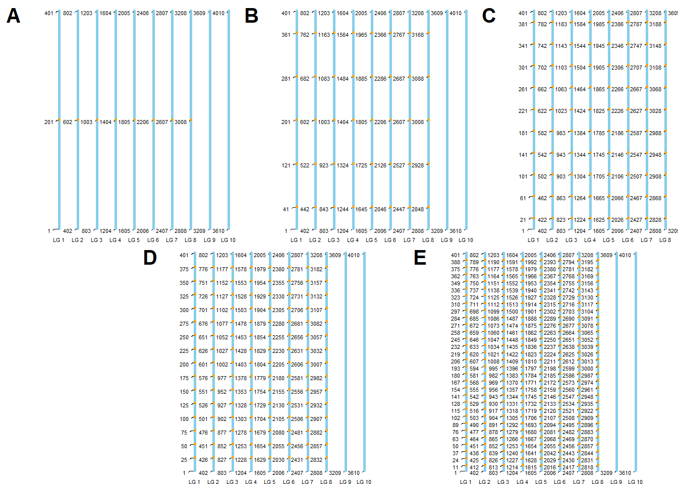

Past versions of unnamed-chunk-7-1.png

Version	Author	Date
492212b	WevertonGomesCosta	2025-03-24

Session information

sessionInfo()

R version 4.4.3 (2025-02-28 ucrt)
Platform: x86_64-w64-mingw32/x64
Running under: Windows 11 x64 (build 26100)

Matrix products: default


locale:
[1] LC_COLLATE=Portuguese_Brazil.utf8  LC_CTYPE=Portuguese_Brazil.utf8   
[3] LC_MONETARY=Portuguese_Brazil.utf8 LC_NUMERIC=C                      
[5] LC_TIME=Portuguese_Brazil.utf8    

time zone: America/Sao_Paulo
tzcode source: internal

attached base packages:
[1] stats     graphics  grDevices utils     datasets  methods   base     

other attached packages:
 [1] tidytext_0.4.2    cowplot_1.1.3     ggpubr_0.6.0      ggrepel_0.9.6    
 [5] ggthemes_5.1.0    data.table_1.17.0 lubridate_1.9.4   forcats_1.0.0    
 [9] stringr_1.5.1     dplyr_1.1.4       purrr_1.0.4       readr_2.1.5      
[13] tidyr_1.3.1       tibble_3.2.1      ggplot2_3.5.1     tidyverse_2.0.0  

loaded via a namespace (and not attached):
 [1] gtable_0.3.6      xfun_0.51         bslib_0.9.0       rstatix_0.7.2    
 [5] lattice_0.22-6    tzdb_0.4.0        vctrs_0.6.5       tools_4.4.3      
 [9] generics_0.1.3    janeaustenr_1.0.0 tokenizers_0.3.0  pkgconfig_2.0.3  
[13] Matrix_1.7-2      lifecycle_1.0.4   farver_2.1.2      compiler_4.4.3   
[17] git2r_0.35.0      munsell_0.5.1     carData_3.0-5     httpuv_1.6.15    
[21] SnowballC_0.7.1   htmltools_0.5.8.1 sass_0.4.9        yaml_2.3.10      
[25] Formula_1.2-5     later_1.4.1       pillar_1.10.1     car_3.1-3        
[29] jquerylib_0.1.4   whisker_0.4.1     cachem_1.1.0      abind_1.4-8      
[33] tidyselect_1.2.1  digest_0.6.37     stringi_1.8.4     labeling_0.4.3   
[37] rprojroot_2.0.4   fastmap_1.2.0     grid_4.4.3        colorspace_2.1-1 
[41] cli_3.6.4         magrittr_2.0.3    broom_1.0.7       withr_3.0.2      
[45] scales_1.3.0      promises_1.3.2    backports_1.5.0   timechange_0.3.0 
[49] rmarkdown_2.29    ggsignif_0.6.4    workflowr_1.7.1   hms_1.1.3        
[53] evaluate_1.0.3    knitr_1.49        rlang_1.1.5       Rcpp_1.0.14      
[57] glue_1.8.0        rstudioapi_0.17.1 jsonlite_1.9.1    R6_2.6.1         
[61] fs_1.6.5