Last updated: 2025-01-21
Checks: 6 1
Knit directory:
Genomic-Selection-for-Drought-Tolerance-Using-Genome-Wide-SNPs-in-Casava/
This reproducible R Markdown analysis was created with workflowr (version 1.7.1). The Checks tab describes the reproducibility checks that were applied when the results were created. The Past versions tab lists the development history.
The R Markdown file has unstaged changes. To know which version of
the R Markdown file created these results, you’ll want to first commit
it to the Git repo. If you’re still working on the analysis, you can
ignore this warning. When you’re finished, you can run
wflow_publish to commit the R Markdown file and build the
HTML.
Great job! The global environment was empty. Objects defined in the global environment can affect the analysis in your R Markdown file in unknown ways. For reproduciblity it’s best to always run the code in an empty environment.
The command set.seed(20221020) was run prior to running
the code in the R Markdown file. Setting a seed ensures that any results
that rely on randomness, e.g. subsampling or permutations, are
reproducible.
Great job! Recording the operating system, R version, and package versions is critical for reproducibility.
Nice! There were no cached chunks for this analysis, so you can be confident that you successfully produced the results during this run.
Great job! Using relative paths to the files within your workflowr project makes it easier to run your code on other machines.
Great! You are using Git for version control. Tracking code development and connecting the code version to the results is critical for reproducibility.
The results in this page were generated with repository version d3a1229. See the Past versions tab to see a history of the changes made to the R Markdown and HTML files.
Note that you need to be careful to ensure that all relevant files for
the analysis have been committed to Git prior to generating the results
(you can use wflow_publish or
wflow_git_commit). workflowr only checks the R Markdown
file, but you know if there are other scripts or data files that it
depends on. Below is the status of the Git repository when the results
were generated:
Ignored files:
    Ignored:    .Rhistory
    Ignored:    .Rproj.user/
    Ignored:    analysis/figure/GWS.Rmd/
    Ignored:    analysis/figure/clone_selection.Rmd/
    Ignored:    data/Artigo/
    Ignored:    data/allchrAR08.txt
    Ignored:    data/data.rar
    Ignored:    data/geno.rds
    Ignored:    data/pheno.rds
    Ignored:    output/BLUPS_density_med_row_col.png
    Ignored:    output/GEBVS_BayesA.RDS
    Ignored:    output/GEBVS_BayesB.RDS
    Ignored:    output/GEBVS_DOM.RDS
    Ignored:    output/GEBVS_G_BLUP.RDS
    Ignored:    output/GEBVS_RF.RDS
    Ignored:    output/GEBVS_RKHS.RDS
    Ignored:    output/GEBVS_RR_BLUP.RDS
    Ignored:    output/G_matrix.rds
    Ignored:    output/accuracy_all_methods.tiff
    Ignored:    output/indice_selection_GEBV_GETGV.tiff
    Ignored:    output/kappa.tiff
    Ignored:    output/result_sommer_row_col_random.RDS
    Ignored:    output/results_cv_BayesA.RDS
    Ignored:    output/results_cv_BayesB.RDS
    Ignored:    output/results_cv_GEBVS_DOM.RDS
    Ignored:    output/results_cv_G_BLUP.RDS
    Ignored:    output/results_cv_RF.RDS
    Ignored:    output/results_cv_RKHS.RDS
    Ignored:    output/results_cv_RR_BLUP.RDS

Unstaged changes:
    Modified:   analysis/clone_selection.Rmd
    Deleted:    data/~WRL2427.tmp
    Modified:   output/dierencial_selecao.csv
    Modified:   output/results_kappa.csv
Note that any generated files, e.g. HTML, png, CSS, etc., are not included in this status report because it is ok for generated content to have uncommitted changes.
These are the previous versions of the repository in which changes were
made to the R Markdown (analysis/clone_selection.Rmd) and
HTML (docs/clone_selection.html) files. If you’ve
configured a remote Git repository (see ?wflow_git_remote),
click on the hyperlinks in the table below to view the files as they
were in that past version.
| File | Version | Author | Date | Message |
|---|---|---|---|---|
| Rmd | 6ba1257 | Weverton Gomes | 2025-01-20 | Commitar todas as mudanças antes de reescrever o histórico |
| html | 6ba1257 | Weverton Gomes | 2025-01-20 | Commitar todas as mudanças antes de reescrever o histórico |
Configurations and packages
To perform the analyses, we will need the following packages:
Data
results <- readRDS("output/results_cv_G_BLUP.RDS") %>%
  mutate(method = "G-BLUP") %>%
  bind_rows(
    readRDS("output/results_cv_RR_BLUP.RDS") %>%
      mutate(method = "RR-BLUP"),
    readRDS("output/results_cv_RKHS.RDS") %>%
      mutate(method = "RKHS"),
    readRDS("output/results_cv_BayesA.RDS") %>%
      mutate(method = "Bayes A"),
    readRDS("output/results_cv_BayesB.RDS") %>%
      mutate(method = "Bayes B"),
    readRDS("output/results_cv_RF.RDS") %>%
      mutate(method = "RF"),
    readRDS("output/results_cv_GEBVS_DOM.RDS") %>%
      mutate(method = "G-BLUP-DOM")
  )

traits <- unique(results$Trait)
Results
Plot boxplot from Accuracy
Figure 2 Boxplot of predictive ability
results %>%
  ggplot(aes(x = method, y = Ac, fill = method)) +
  geom_boxplot() +
  facet_wrap(~ Trait, ncol = 6) +
  expand_limits(y = 0) +
  labs(y = "Accuracy", x = "", fill = "Method") +
  scale_fill_gdocs() +
  theme(
    text = element_text(size = 25),
    axis.text.x = element_blank(),
    axis.ticks.x = element_blank(),
    legend.position = "top",
    legend.title = element_blank(),
    legend.box = "horizontal",
    panel.spacing = unit(1, "lines"),
    strip.background = element_blank(),
    panel.background = element_blank(),
    plot.background = element_blank(),
    legend.background = element_blank(),
    legend.box.background = element_blank(),
    legend.key = element_blank()
  ) +
  guides(fill = guide_legend(
    nrow = 1,
    byrow = TRUE,
    keywidth = 1.5,
    keyheight = 1,
    title.position = "top"
  ))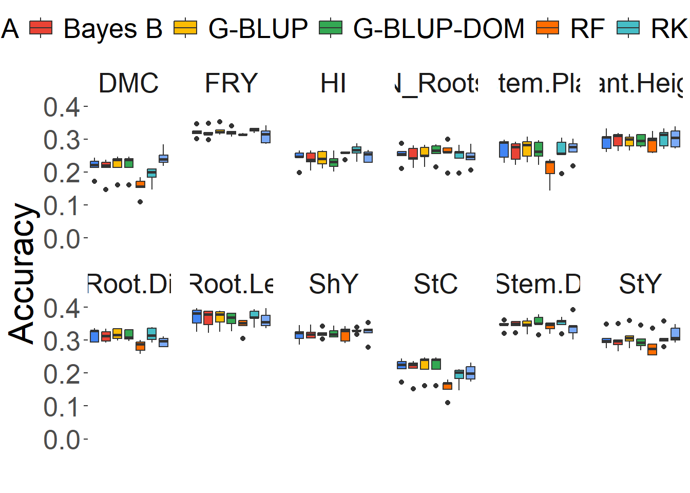
Table to Figure 2 Boxplot of predictive ability
# Calcular médias e desvio padrão de Ac por Trait e método
results_Ac <- results %>%
  group_by(Trait, method) %>%
  summarise(
    Ac_mean = round(mean(Ac) * 100, 2),
    Ac_sd = round(sd(Ac) * 100, 2),
    .groups = "drop"  # Remove agrupamento após summarise
  ) %>%
  select(Trait, method, Ac_mean) %>%
  pivot_wider(names_from = method, values_from = Ac_mean)

# Exibir resultados em tabela com kable
results_Ac %>%
  kbl(escape = FALSE, align = "c") %>%
  kable_classic(
    "hover",
    full_width = FALSE,
    position = "center",
    fixed_thead = TRUE
)| Trait | Bayes A | Bayes B | G-BLUP | G-BLUP-DOM | RF | RKHS | RR-BLUP |
|---|---|---|---|---|---|---|---|
| DMC | 21.64 | 20.94 | 22.00 | 22.00 | 15.48 | 19.00 | 24.46 |
| FRY | 32.22 | 31.94 | 32.66 | 32.10 | 31.40 | 32.80 | 31.16 |
| HI | 24.26 | 23.90 | 24.06 | 23.08 | 25.54 | 26.40 | 24.78 |
| N_Roots | 25.28 | 24.94 | 25.42 | 26.02 | 25.78 | 24.84 | 24.62 |
| Nstem.Plant | 27.08 | 26.28 | 27.22 | 26.40 | 20.82 | 26.00 | 26.84 |
| Plant.Height | 29.58 | 29.72 | 29.32 | 29.56 | 28.86 | 30.32 | 30.30 |
| Root.Di | 31.60 | 31.28 | 31.80 | 31.50 | 28.24 | 31.70 | 29.48 |
| Root.Le | 36.94 | 36.54 | 36.72 | 36.24 | 34.46 | 37.14 | 36.16 |
| ShY | 31.76 | 32.02 | 32.10 | 32.16 | 31.82 | 32.88 | 32.40 |
| StC | 21.80 | 21.16 | 22.12 | 22.12 | 15.56 | 19.08 | 20.12 |
| StY | 30.44 | 30.04 | 31.04 | 29.86 | 28.18 | 30.90 | 31.70 |
| Stem.D | 34.58 | 34.64 | 34.68 | 35.34 | 34.12 | 35.12 | 34.02 |
# Calcular médias e desvio padrão de MSPE por Trait e método
results_MSPE <- results %>%
  group_by(Trait, method) %>%
  summarise(
    MSPE_mean = round(mean(MSPE) * 100, 2),
    MSPE_sd = round(sd(MSPE) * 100, 2),
    .groups = "drop"  # Remove agrupamento após summarise
  ) %>%
  select(Trait, method, MSPE_mean) %>%
  pivot_wider(names_from = method, values_from = MSPE_mean)

# Exibir resultados em tabela com kable
results_MSPE %>%
  kbl(escape = FALSE, align = "c") %>%
  kable_classic(
    "hover",
    full_width = FALSE,
    position = "center",
    fixed_thead = TRUE
)| Trait | Bayes A | Bayes B | G-BLUP | G-BLUP-DOM | RF | RKHS | RR-BLUP |
|---|---|---|---|---|---|---|---|
| DMC | 589.82 | 593.86 | 585.32 | 585.32 | 628.74 | 611.50 | 576.84 |
| FRY | 115.86 | 116.34 | 115.26 | 116.12 | 117.38 | 119.72 | 116.66 |
| HI | 1195.86 | 1199.12 | 1189.96 | 1198.26 | 1212.24 | 1176.24 | 1186.60 |
| N_Roots | 86.08 | 86.14 | 85.74 | 85.48 | 87.68 | 93.12 | 88.26 |
| Nstem.Plant | 2.76 | 2.80 | 2.76 | 2.78 | 2.98 | 3.30 | 2.88 |
| Plant.Height | 0.74 | 0.74 | 0.74 | 0.74 | 0.78 | 0.80 | 0.78 |
| Root.Di | 332.88 | 333.62 | 332.10 | 332.84 | 348.66 | 339.12 | 338.06 |
| Root.Le | 180.68 | 181.42 | 180.78 | 181.48 | 187.28 | 198.94 | 199.96 |
| ShY | 1259.58 | 1257.72 | 1253.94 | 1254.40 | 1276.28 | 1324.08 | 1261.50 |
| StC | 586.66 | 589.94 | 582.36 | 582.36 | 625.52 | 608.10 | 591.46 |
| StY | 7.08 | 7.10 | 7.02 | 7.10 | 7.24 | 7.24 | 7.02 |
| Stem.D | 0.78 | 0.76 | 0.76 | 0.76 | 0.80 | 0.84 | 0.80 |
Clone Selection
First let’s add the phenotypic means to the BLUPS and GEBVS
# Carregar dados
media_pheno <- read.csv("output/mean_pheno.csv")

BLUPS <- readRDS("data/pheno.rds") %>%
  pivot_longer(cols = -ID_Clone, names_to = "Trait", values_to = "BLUP")

# Inserir o método em cada data frame dentro de results$result
results$result <- map2(results$result, results$method, ~mutate(.x, method = .y))

# Combinar todos os data frames em um único data frame
GEBV_BLUP <- bind_rows(results$result) %>%
  group_by(ID_Clone, Trait, method) %>%
  summarise(GEBV = mean(GEBV), .groups = "drop") %>%
  pivot_wider(names_from = method, values_from = GEBV) %>%
  full_join(BLUPS, by = c("ID_Clone", "Trait"))

# Adicionar as médias fenotípicas aos valores numéricos e combinar com GEBV
GEBV_BLUP <- GEBV_BLUP %>%
  rowwise() %>%
  mutate(across(where(is.numeric), ~ . + media_pheno[[Trait]])) %>%
  ungroup()

# Visualizar os primeiros dados
GEBV_BLUP %>%
  head() %>%
  kbl(escape = FALSE, align = "c") %>%
kable_classic("hover", full_width = FALSE, position = "center", fixed_thead = TRUE)| ID_Clone | Trait | Bayes A | Bayes B | G-BLUP | G-BLUP-DOM | RF | RKHS | RR-BLUP | BLUP |
|---|---|---|---|---|---|---|---|---|---|
| Alagoana363.250437472 | FRY | 5.147048 | 5.136213 | 5.188144 | 5.255897 | 5.275877 | 5.432111 | 5.225135 | 4.980623 |
| Alagoana363.250437472 | HI | 24.607030 | 24.568547 | 24.633235 | 24.672048 | 24.723454 | 24.444491 | 25.165928 | 24.557231 |
| Alagoana363.250437472 | N_Roots | 4.154301 | 4.178224 | 4.225263 | 4.243897 | 4.193898 | 4.443810 | 4.426670 | 3.958834 |
| Alagoana363.250437472 | Plant.Height | 1.161012 | 1.161261 | 1.160419 | 1.165587 | 1.165375 | 1.187893 | 1.175966 | 1.170988 |
| Alagoana363.250437472 | Root.Di | 29.609365 | 29.596120 | 29.557053 | 29.568693 | 30.003957 | 29.749311 | 29.896532 | 30.209694 |
| Alagoana363.250437472 | Root.Le | 23.563618 | 23.558956 | 23.535616 | 23.534217 | 23.494775 | 23.850965 | 23.866019 | 23.341948 |
Now let’s group the BLUPs data with the GEBVs and GETGVs data and add a Weights column for each increase or decrease characteristic.
selection_parents <- GEBV_BLUP %>%
  rename(GEBV = `G-BLUP`, GETGV = `G-BLUP-DOM`) |>
  mutate(Weights = ifelse(
    Trait %in% traits,
    "acrescimo",
    "descrescimo"
  ))

calcular_pesos <- function(data, var){
  selection_parents  %>%
  select(ID_Clone, Trait, all_of(var)) %>%
  pivot_wider(names_from = Trait, values_from = all_of(var)) %>%
  mutate(
    N_Roots = 15 * N_Roots,
    FRY = 20 * FRY,
    ShY = 10 * ShY,
    DMC = 15 * DMC,
    StY = 10 * StY,
    Plant.Height = 5 * Plant.Height,
    HI = 10 * HI,
    StC = 10 * StC,
    Root.Le = 5 * Root.Le,
    Root.Di = 5 * Root.Di,
    Stem.D = 5 * Stem.D,
    Nstem.Plant = 5 * Nstem.Plant
  ) %>%
  mutate(pesos =
           rowSums(.[2:13], na.rm = TRUE))
}

pesos_BLUP <- calcular_pesos(selection_parents, "BLUP")
pesos_GEBV <- calcular_pesos(selection_parents, "GEBV")
pesos_GETGV <- calcular_pesos(selection_parents, "GETGV")
Individual selection to each trait
results_kappa <- data.frame()
SI <- c(10, 15, 20, 25, 30)

clones_sel_pesos <- function(pesos) {
  pesos %>%
    right_join(sel_parents) %>%
    droplevels() %>%
    arrange(desc(pesos)) %>%
    slice(1:(nlevels(ID_Clone) * (i / 100))) |>
    droplevels()
}

clone_sel_method <- function(data, method) {
  data %>%
    # Use a `mutate` para criar uma coluna temporária que armazena os valores de ordenação
    mutate(OrderingValue = ifelse(Weights == "acrescimo", get(method), -get(method))) %>%
    arrange(desc(OrderingValue)) %>%
    slice(1:(nlevels(ID_Clone) * (i / 100))) %>%
    droplevels() %>%
    select(-OrderingValue)  # Remova a coluna temporária
}

comb_sel <- function(var1, var2) {
  get(paste0("Clones_sel_", var1)) %>%
    full_join(get(paste0("Clones_sel_", var2))) %>%
    resca(BLUP, GEBV, GETGV, new_min = 0, new_max = 1) %>%
    mutate(!!paste0(var1, "_", var2) := (get(paste0(var1, "_res")) + get(paste0(var2, "_res"))) / 2) %>%
    arrange(desc(get(paste0(var1, "_", var2)))) %>%
    slice(1:nrow(Clones_sel_BLUP)) %>%
    droplevels()
}

calcular_media <- function(data, var) {
  data %>%
    filter(Trait == j) %>%
    select(all_of(var)) %>%
    summarise(mean(.[[1]], na.rm = T)) %>%
    pull()
}

calcular_media_sel <- function(data, var) {
  get(paste0("Clones_sel_", var)) %>%
    filter(Trait == j &
             ID_Clone %in% get(paste0("Clones_", var, "_sel"))$ID_Clone) %>%
    select(all_of(var)) %>%
    summarise(mean(.[[1]], na.rm = T)) %>%
    pull()
}

calcular_media_comb_sel <- function(data, var1, var2) {
  data %>%
    filter(Trait == j &
             ID_Clone %in% get(paste0("Comb_sel_", var1, "_", var2))$ID_Clone) %>%
    select(all_of(var1)) %>%
    summarise(mean(.[[1]], na.rm = T)) %>%
    pull()
}

# Função para calcular kappa
calcular_kappa <- function(var1, var2) {
  cohen.kappa(cbind(Clones_sel[[var1]], Clones_sel[[var2]]))[["kappa"]]
}
# Melhore a clareza e a eficiência do loop de seleção
for (j in traits) {
for (i in SI) {
sel_parents <- droplevels(na.omit(subset(selection_parents, Trait == j)))
# Aplicar a função clones_sel_pesos para selecionar clones
Clones_GEBV_sel <- clones_sel_pesos(pesos_GEBV)
Clones_GETGV_sel <- clones_sel_pesos(pesos_GETGV)
Clones_BLUP_sel <- clones_sel_pesos(pesos_BLUP)
# Aplicar a função clone_sel_method para métodos de seleção
Clones_sel_BLUP <- clone_sel_method(sel_parents, "BLUP")
Clones_sel_GEBV <- clone_sel_method(sel_parents, "GEBV")
Clones_sel_GETGV <- clone_sel_method(sel_parents, "GETGV")
# Calcular médias
X0_BLUPS <- calcular_media(selection_parents, "BLUP")
X0_GEBV <- calcular_media(selection_parents, "GEBV")
X0_GETGV <- calcular_media(selection_parents, "GETGV")
XS_BLUPS <- calcular_media_sel(Clones_sel_BLUP, "BLUP")
XS_GEBV <- calcular_media_sel(Clones_sel_GEBV, "GEBV")
XS_GETGV <- calcular_media_sel(Clones_sel_GETGV, "GETGV")
# Combinar seleções
Comb_sel_GEBV_BLUP <- comb_sel("GEBV", "BLUP")
Comb_sel_GETGV_BLUP <- comb_sel("GETGV", "BLUP")
Comb_sel_GETGV_GEBV <- comb_sel("GETGV", "GEBV")
# Calcular médias combinadas
XS_GEBV_BLUP <- calcular_media_comb_sel(selection_parents, "GEBV", "BLUP")
XS_GETGV_BLUP <- calcular_media_comb_sel(selection_parents, "GETGV", "BLUP")
XS_GETGV_GEBV <- calcular_media_comb_sel(selection_parents, "GETGV", "GEBV")
# Selecionar clones
Clones_sel <- transform(BLUPS,
BLUPS_sel = as.integer(ID_Clone %in% Clones_sel_BLUP$ID_Clone),
GEBVS_sel = as.integer(ID_Clone %in% Clones_sel_GEBV$ID_Clone),
GETGV_sel = as.integer(ID_Clone %in% Clones_sel_GETGV$ID_Clone),
Comb_sel_GEBV_BLUP = as.integer(ID_Clone %in% Comb_sel_GEBV_BLUP$ID_Clone),
Comb_sel_GETGV_BLUP = as.integer(ID_Clone %in% Comb_sel_GETGV_BLUP$ID_Clone),
Comb_sel_GETGV_GEBV = as.integer(ID_Clone %in% Comb_sel_GETGV_GEBV$ID_Clone))
# Calcular valores de kappa
kappa_values <- data.frame(
kappa_GEBV_BLUP = calcular_kappa("BLUPS_sel", "GEBVS_sel"),
kappa_GETGV_BLUP = calcular_kappa("BLUPS_sel", "GETGV_sel"),
kappa_GETGV_GEBV = calcular_kappa("GEBVS_sel", "GETGV_sel"),
kappa_sel_GEBV_BLUP_BLUP = calcular_kappa("BLUPS_sel", "Comb_sel_GEBV_BLUP"),
kappa_sel_GETGV_BLUP_BLUP = calcular_kappa("BLUPS_sel", "Comb_sel_GETGV_BLUP"),
kappa_sel_GETGV_GEBV_BLUP = calcular_kappa("BLUPS_sel", "Comb_sel_GETGV_GEBV"),
kappa_sel_GEBV_BLUP_GEBV = calcular_kappa("GEBVS_sel", "Comb_sel_GEBV_BLUP"),
kappa_sel_GETGV_BLUP_GEBV = calcular_kappa("GEBVS_sel", "Comb_sel_GETGV_BLUP"),
kappa_sel_GETGV_GEBV_GEBV = calcular_kappa("GEBVS_sel", "Comb_sel_GETGV_GEBV"),
kappa_sel_GEBV_BLUP_GETGV = calcular_kappa("GETGV_sel", "Comb_sel_GEBV_BLUP"),
kappa_sel_GETGV_BLUP_GETGV = calcular_kappa("GETGV_sel", "Comb_sel_GETGV_BLUP"),
kappa_sel_GETGV_GEBV_GETGV = calcular_kappa("GETGV_sel", "Comb_sel_GETGV_GEBV")
)
# Coeficientes kappa
coef_kappa <- data.frame(
Trait = j,
SI = i,
X0 = media_pheno[[j]],
X0_GEBV,
X0_GETGV,
X0_BLUPS,
XS_BLUPS,
XS_GEBV,
XS_GETGV,
XS_GEBV_BLUP,
XS_GETGV_BLUP,
XS_GETGV_GEBV
)
coef_kappa <- cbind(coef_kappa, kappa_values)
# Anexar os resultados
results_kappa <- rbind(results_kappa, coef_kappa)
}
}Figure 3 Cohen’s Kappa of coincidence
results_kappa |>
  pivot_longer(names_to = "Comparation",
               values_to = "Kappa",
               cols = 13:18) %>%
  ggplot(aes(x = Trait, y = SI, fill = Kappa)) +
  geom_tile() +
  facet_wrap(Comparation ~ ., labeller = as_labeller(
    c(
      kappa_GEBV_BLUP = "GEBV x BLUP",
      kappa_GETGV_BLUP = "GETGV x BLUP",
      kappa_GETGV_GEBV = "GEBV x GETGV",
      kappa_sel_GEBV_BLUP_BLUP = "GEBV_BLUP x BLUP",
      kappa_sel_GETGV_BLUP_BLUP = "GETGV_BLUP x BLUP",
      kappa_sel_GETGV_GEBV_BLUP = "GETGV_GEBV x BLUP"
    )
  ), ncol = 2) +
  scale_fill_viridis(discrete = FALSE, limits = c(-0.07, 1)) +
  labs(x = "" , y = "Selection Index", fill = "Kappa") +
  theme_bw() +
  theme(
    text = element_text(size = 20),
    legend.key.width = unit(1.5, 'cm'),
    legend.box = "horizontal",
    legend.position = "top",
    legend.background =  element_blank(),
    strip.background = element_blank(),
    panel.background = element_blank(),
    plot.background = element_blank(),
    axis.text.x = element_text(
      angle = 45,
      hjust = 1,
      vjust = 1
    )
  )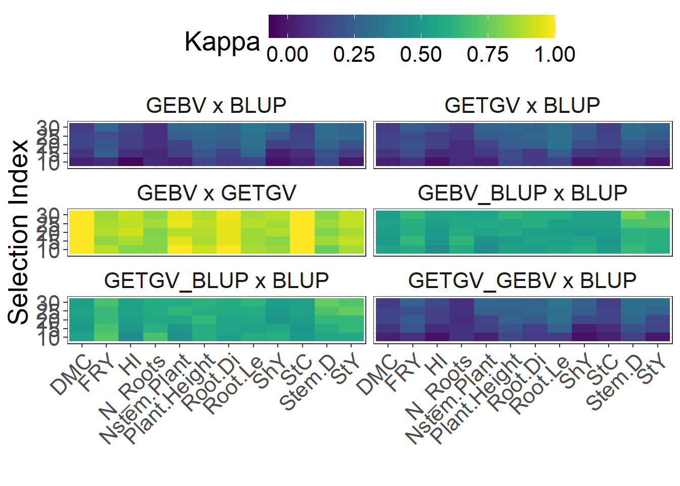
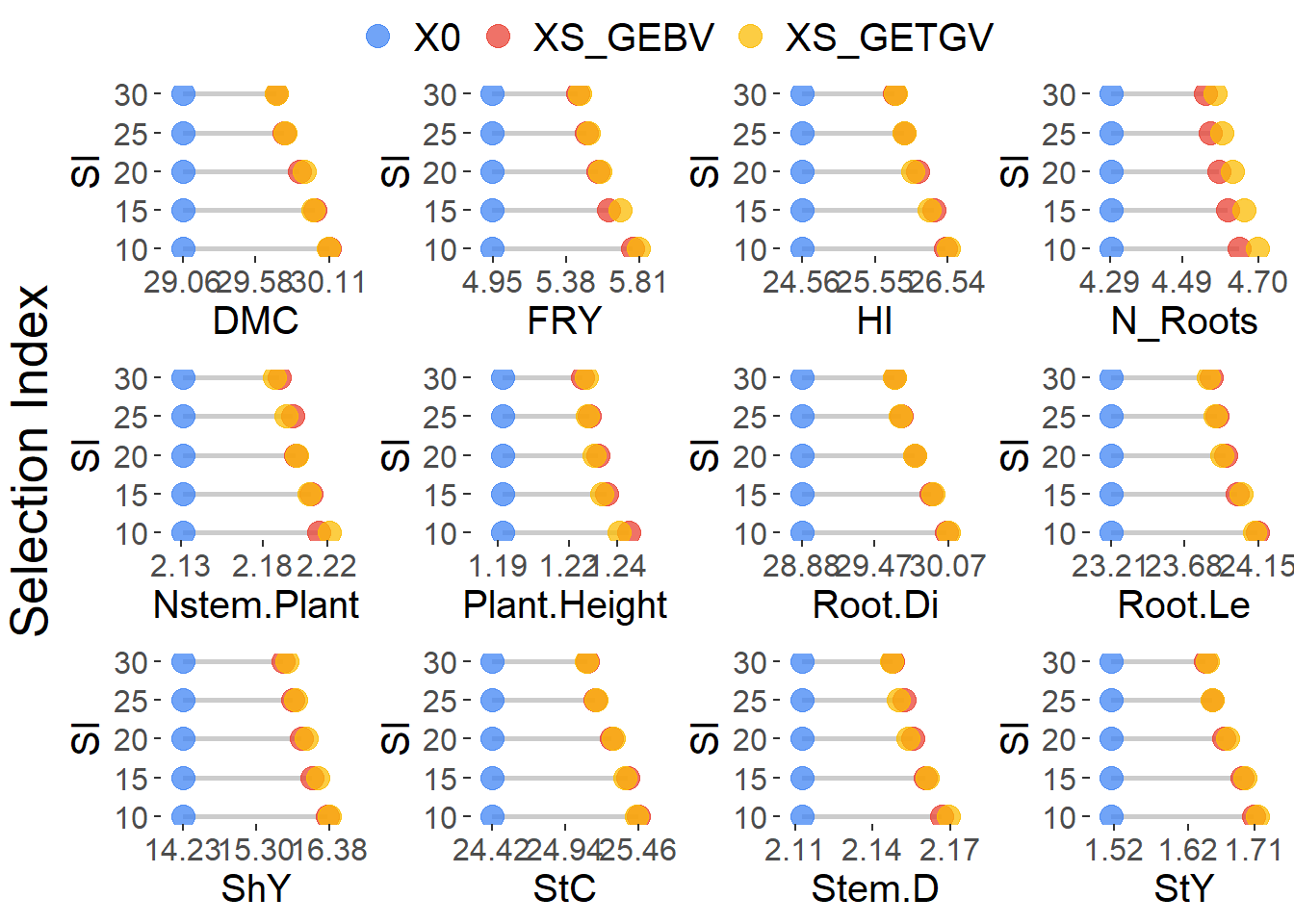
Figure 4: Selection gains
teste <-  results_kappa %>%
  select(Trait, SI, X0, XS_GEBV, XS_GETGV)

p <- list()

for (i in levels(factor(teste$Trait))) {
  breaks <- teste %>%
    filter(Trait == i) %>%
    droplevels() %>%
    group_by(Trait) %>%
    summarise(
      min_X0 = min(X0),
      max_XS = max(c(XS_GEBV, XS_GETGV)),
      mean_X0_XS = mean(c(min_X0, max_XS))
    ) %>%
    round_cols()

  p[[i]] <- teste %>%
    filter(Trait == i) %>%
    droplevels() %>%
    ggplot(aes(y = SI,
               x = start)) +
    geom_segment(
      aes(
        x = X0,
        xend = XS_GEBV,
        y = SI,
        yend = SI
      ),
      linewidth = 1,
      color = "gray80"
    ) +
    geom_point(
      data = teste %>%
        filter(Trait == i) %>%
        droplevels() %>%
        pivot_longer(
          names_to = "measure",
          values_to = "value",
          cols = c("X0", "XS_GEBV", "XS_GETGV")
        ),
      aes(y = SI,
          x = value,
          color = measure),
      size = 4,
      alpha = 0.75
    )  +
    scale_x_continuous(
      limits = ~ c(min(.x), max(.x)),
      breaks = c(breaks$min_X0, breaks$mean_X0_XS, breaks$max_XS),
      expand = expansion(mult = ifelse(i == "Plant.Height" , 0.25, 0.15))
    ) +
    scale_color_gdocs() +
    labs(x = i)  +
    theme(
      text = element_text(size = 15),
      legend.text = element_text(size = 15),
      legend.box = "horizontal",
      legend.direction = "horizontal",
      legend.position = "top",
      panel.spacing = unit(2, "lines"),
      legend.title = element_blank(),
      panel.background = element_blank(),
      panel.border = element_blank(),
      plot.background = element_blank(),
      legend.background = element_blank(),
      legend.box.background = element_blank(),
      legend.key = element_blank()
    )
}

annotate_figure(
  ggarrange(
    plotlist = p,
    nrow = 3,
    ncol = 4,
    common.legend = TRUE),
  left = text_grob("Selection Index", rot = 90, size = 20)
)
Supplementary Table 3 - Cohen’s Kappa of coincidence
results_kappa |>
  select(1,2, starts_with("kappa")) %>%
  kbl(escape = F, align = 'c') |>
kable_classic("hover", full_width = F, position = "center", fixed_thead = T)| Trait | SI | kappa_GEBV_BLUP | kappa_GETGV_BLUP | kappa_GETGV_GEBV | kappa_sel_GEBV_BLUP_BLUP | kappa_sel_GETGV_BLUP_BLUP | kappa_sel_GETGV_GEBV_BLUP | kappa_sel_GEBV_BLUP_GEBV | kappa_sel_GETGV_BLUP_GEBV | kappa_sel_GETGV_GEBV_GEBV | kappa_sel_GEBV_BLUP_GETGV | kappa_sel_GETGV_BLUP_GETGV | kappa_sel_GETGV_GEBV_GETGV |
|---|---|---|---|---|---|---|---|---|---|---|---|---|---|
| N_Roots | 10 | 0.0593333 | 0.0593333 | 0.8063333 | 0.5850000 | 0.6956667 | 0.0870000 | 0.4743333 | 0.3360000 | 0.9170000 | 0.3913333 | 0.3636667 | 0.8893333 |
| N_Roots | 15 | 0.0453052 | 0.0647887 | 0.8051643 | 0.6298122 | 0.6103286 | 0.0842723 | 0.4154930 | 0.3960094 | 0.8830986 | 0.3765258 | 0.4544601 | 0.9025822 |
| N_Roots | 20 | 0.0796185 | 0.0642788 | 0.8005840 | 0.5858283 | 0.5704887 | 0.0642788 | 0.4937902 | 0.4784505 | 0.9233015 | 0.4017521 | 0.4937902 | 0.8772825 |
| N_Roots | 25 | 0.0709151 | 0.1101722 | 0.8560573 | 0.5681718 | 0.5812575 | 0.0840008 | 0.5027433 | 0.4634862 | 0.9345715 | 0.5027433 | 0.5289147 | 0.9214858 |
| N_Roots | 30 | 0.0784000 | 0.1133974 | 0.8250126 | 0.5566987 | 0.5800304 | 0.0784000 | 0.5217012 | 0.4750379 | 0.9066734 | 0.5450329 | 0.5333671 | 0.9183392 |
| FRY | 10 | 0.0593333 | 0.0870000 | 0.8893333 | 0.5850000 | 0.7233333 | 0.0870000 | 0.4743333 | 0.3360000 | 0.9446667 | 0.5020000 | 0.3636667 | 0.9446667 |
| FRY | 15 | 0.2312679 | 0.1736130 | 0.8270353 | 0.6348523 | 0.6925072 | 0.2120496 | 0.5964157 | 0.5195425 | 0.9231268 | 0.5387608 | 0.4811059 | 0.9039085 |
| FRY | 20 | 0.2176758 | 0.2023361 | 0.8772825 | 0.6011680 | 0.6471871 | 0.2330155 | 0.6165077 | 0.5704887 | 0.9693206 | 0.6011680 | 0.5551490 | 0.9079619 |
| FRY | 25 | 0.1886864 | 0.1756007 | 0.8691430 | 0.5943432 | 0.6466860 | 0.1886864 | 0.5943432 | 0.5420004 | 0.9345715 | 0.5681718 | 0.5289147 | 0.9345715 |
| FRY | 30 | 0.2801992 | 0.2453701 | 0.8490740 | 0.6400996 | 0.6865384 | 0.2685895 | 0.6400996 | 0.5820511 | 0.9419515 | 0.6052705 | 0.5588318 | 0.9071225 |
| ShY | 10 | -0.0284335 | -0.0013695 | 0.8376158 | 0.5940394 | 0.5940394 | -0.0284335 | 0.3775271 | 0.3504630 | 0.9458719 | 0.2963349 | 0.4045911 | 0.8917438 |
| ShY | 15 | 0.0198666 | 0.0967398 | 0.8078170 | 0.5579791 | 0.5579791 | 0.0198666 | 0.4618876 | 0.4234510 | 0.9039085 | 0.4811059 | 0.5387608 | 0.9039085 |
| ShY | 20 | 0.1337069 | 0.1793013 | 0.8784150 | 0.5136600 | 0.4984619 | 0.1641031 | 0.6200469 | 0.6352450 | 0.9088113 | 0.6352450 | 0.6808394 | 0.9696038 |
| ShY | 25 | 0.2251680 | 0.2380819 | 0.8579475 | 0.5480147 | 0.5092731 | 0.2380819 | 0.6771533 | 0.7029811 | 0.9483445 | 0.6771533 | 0.7288088 | 0.9096029 |
| ShY | 30 | 0.2951609 | 0.2258325 | 0.8844526 | 0.5378104 | 0.5262557 | 0.2489420 | 0.7573505 | 0.7342410 | 0.9537810 | 0.6880221 | 0.6995768 | 0.9306716 |
| DMC | 10 | 0.0238575 | 0.0238575 | 1.0000000 | 0.5467910 | 0.5467910 | 0.0238575 | 0.4770665 | 0.4770665 | 1.0000000 | 0.4770665 | 0.4770665 | 1.0000000 |
| DMC | 15 | 0.0953812 | 0.0953812 | 1.0000000 | 0.5110168 | 0.5110168 | 0.0953812 | 0.5843643 | 0.5843643 | 1.0000000 | 0.5843643 | 0.5843643 | 1.0000000 |
| DMC | 20 | 0.1467148 | 0.1467148 | 1.0000000 | 0.5259527 | 0.5259527 | 0.1467148 | 0.6207621 | 0.6207621 | 1.0000000 | 0.6207621 | 0.6207621 | 1.0000000 |
| DMC | 25 | 0.1389380 | 0.1389380 | 1.0000000 | 0.5375778 | 0.5375778 | 0.1389380 | 0.6013602 | 0.6013602 | 1.0000000 | 0.6013602 | 0.6013602 | 1.0000000 |
| DMC | 30 | 0.1130702 | 0.1130702 | 1.0000000 | 0.5288185 | 0.5288185 | 0.1130702 | 0.5842517 | 0.5842517 | 1.0000000 | 0.5842517 | 0.5842517 | 1.0000000 |
| StY | 10 | -0.0060606 | -0.0060606 | 0.8562771 | 0.6047619 | 0.5688312 | -0.0060606 | 0.3891775 | 0.4251082 | 0.9281385 | 0.3891775 | 0.4251082 | 0.9281385 |
| StY | 15 | 0.1198303 | 0.1198303 | 0.9022034 | 0.6088135 | 0.6332626 | 0.1442795 | 0.5110168 | 0.4865677 | 0.9266525 | 0.5110168 | 0.4865677 | 0.9755508 |
| StY | 20 | 0.1928313 | 0.1736130 | 0.8654719 | 0.6156340 | 0.6348523 | 0.1543947 | 0.5771974 | 0.5579791 | 0.9423451 | 0.5579791 | 0.5387608 | 0.9231268 |
| StY | 25 | 0.2824483 | 0.2346115 | 0.9043264 | 0.7129793 | 0.7448705 | 0.2665027 | 0.5694690 | 0.5375778 | 0.9681088 | 0.5216322 | 0.4897410 | 0.9202720 |
| StY | 30 | 0.2737919 | 0.2737919 | 0.9022412 | 0.6927581 | 0.7067237 | 0.3017230 | 0.5810338 | 0.5670682 | 0.9581034 | 0.5810338 | 0.5670682 | 0.9441378 |
| Plant.Height | 10 | 0.1610147 | 0.1610147 | 0.9188079 | 0.5399113 | 0.5940394 | 0.1610147 | 0.6211034 | 0.5399113 | 0.9729360 | 0.5669753 | 0.5669753 | 0.9458719 |
| Plant.Height | 15 | 0.2120496 | 0.1736130 | 0.8654719 | 0.5195425 | 0.5964157 | 0.2120496 | 0.6925072 | 0.5579791 | 0.9615634 | 0.6156340 | 0.5771974 | 0.9039085 |
| Plant.Height | 20 | 0.2552919 | 0.2400938 | 0.8784150 | 0.5744525 | 0.6352450 | 0.2552919 | 0.6808394 | 0.6200469 | 0.9240094 | 0.6504431 | 0.6048488 | 0.9544056 |
| Plant.Height | 25 | 0.2768235 | 0.2509958 | 0.8966891 | 0.5738424 | 0.5867563 | 0.2509958 | 0.7029811 | 0.6900672 | 0.9612584 | 0.6642395 | 0.6642395 | 0.9354307 |
| Plant.Height | 30 | 0.3067157 | 0.2720515 | 0.8728979 | 0.6302484 | 0.6186936 | 0.2720515 | 0.6764673 | 0.6649126 | 0.9306716 | 0.6302484 | 0.6533578 | 0.9422263 |
| HI | 10 | -0.0513333 | -0.0236667 | 0.8063333 | 0.4466667 | 0.4466667 | -0.0236667 | 0.5020000 | 0.4743333 | 0.8893333 | 0.4743333 | 0.5296667 | 0.9170000 |
| HI | 15 | 0.0775215 | 0.0583032 | 0.8654719 | 0.5003242 | 0.5003242 | 0.0583032 | 0.5771974 | 0.5579791 | 0.9231268 | 0.5387608 | 0.5579791 | 0.9423451 |
| HI | 20 | 0.1256376 | 0.1409773 | 0.9233015 | 0.5091299 | 0.5244696 | 0.1256376 | 0.6165077 | 0.5858283 | 0.9693206 | 0.6318474 | 0.6165077 | 0.9539809 |
| HI | 25 | 0.1363436 | 0.1363436 | 0.8953144 | 0.5289147 | 0.5420004 | 0.1363436 | 0.6074289 | 0.5812575 | 0.9476572 | 0.5943432 | 0.5943432 | 0.9476572 |
| HI | 30 | 0.1524926 | 0.1989313 | 0.9071225 | 0.5588318 | 0.5472221 | 0.1641023 | 0.5936608 | 0.5936608 | 0.9535612 | 0.6168802 | 0.6517093 | 0.9535612 |
| StC | 10 | 0.0238575 | 0.0238575 | 1.0000000 | 0.5119288 | 0.5119288 | 0.0238575 | 0.5119288 | 0.5119288 | 1.0000000 | 0.5119288 | 0.5119288 | 1.0000000 |
| StC | 15 | 0.0709320 | 0.0709320 | 1.0000000 | 0.4865677 | 0.4865677 | 0.0709320 | 0.5843643 | 0.5843643 | 1.0000000 | 0.5843643 | 0.5843643 | 1.0000000 |
| StC | 20 | 0.1467148 | 0.1467148 | 1.0000000 | 0.5259527 | 0.5259527 | 0.1467148 | 0.6207621 | 0.6207621 | 1.0000000 | 0.6207621 | 0.6207621 | 1.0000000 |
| StC | 25 | 0.1389380 | 0.1389380 | 1.0000000 | 0.5375778 | 0.5375778 | 0.1389380 | 0.6013602 | 0.6013602 | 1.0000000 | 0.6013602 | 0.6013602 | 1.0000000 |
| StC | 30 | 0.1269285 | 0.1269285 | 1.0000000 | 0.5426768 | 0.5426768 | 0.1269285 | 0.5842517 | 0.5842517 | 1.0000000 | 0.5842517 | 0.5842517 | 1.0000000 |
| Root.Le | 10 | 0.1423333 | 0.1423333 | 0.8616667 | 0.5573333 | 0.5850000 | 0.1146667 | 0.5850000 | 0.4743333 | 0.9170000 | 0.5296667 | 0.5573333 | 0.9446667 |
| Root.Le | 15 | 0.2791080 | 0.2401408 | 0.8441315 | 0.5323944 | 0.5323944 | 0.2596244 | 0.7467136 | 0.7077465 | 0.9415493 | 0.7077465 | 0.7077465 | 0.9025822 |
| Root.Le | 20 | 0.3250536 | 0.3403933 | 0.8466031 | 0.5244696 | 0.5704887 | 0.3250536 | 0.8005840 | 0.7238856 | 0.9386412 | 0.7852443 | 0.7699046 | 0.9079619 |
| Root.Le | 25 | 0.3326291 | 0.3326291 | 0.8822287 | 0.5420004 | 0.5812575 | 0.3326291 | 0.7906287 | 0.7513716 | 0.9476572 | 0.7644573 | 0.7513716 | 0.9345715 |
| Root.Le | 30 | 0.3583797 | 0.3117164 | 0.8600101 | 0.5916962 | 0.6266937 | 0.3467139 | 0.7666835 | 0.6850228 | 0.9533367 | 0.6966886 | 0.6850228 | 0.8950076 |
| Root.Di | 10 | 0.1146667 | 0.1146667 | 1.0000000 | 0.5296667 | 0.5296667 | 0.1146667 | 0.5850000 | 0.5850000 | 1.0000000 | 0.5850000 | 0.5850000 | 1.0000000 |
| Root.Di | 15 | 0.1427230 | 0.1037559 | 0.9610329 | 0.5518779 | 0.5518779 | 0.1232394 | 0.5908451 | 0.5908451 | 0.9805164 | 0.5518779 | 0.5518779 | 0.9805164 |
| Root.Di | 20 | 0.2330155 | 0.2483551 | 0.9539809 | 0.5398093 | 0.5551490 | 0.2330155 | 0.6932062 | 0.6625268 | 0.9846603 | 0.6932062 | 0.6932062 | 0.9693206 |
| Root.Di | 25 | 0.2672006 | 0.2802863 | 0.9607429 | 0.5943432 | 0.5812575 | 0.2802863 | 0.6728574 | 0.6859431 | 0.9738286 | 0.6859431 | 0.6990288 | 0.9869143 |
| Root.Di | 30 | 0.2650531 | 0.2650531 | 0.9766684 | 0.5916962 | 0.5800304 | 0.2650531 | 0.6733569 | 0.6850228 | 1.0000000 | 0.6733569 | 0.6850228 | 0.9766684 |
| Stem.D | 10 | 0.1610147 | 0.0798226 | 0.7564236 | 0.6481675 | 0.5669753 | 0.1339507 | 0.5128473 | 0.5399113 | 0.8646798 | 0.3775271 | 0.5128473 | 0.8917438 |
| Stem.D | 15 | 0.2036005 | 0.1656767 | 0.8483049 | 0.6207621 | 0.6018002 | 0.2036005 | 0.5828383 | 0.5828383 | 0.9241524 | 0.5069908 | 0.5638765 | 0.9241524 |
| Stem.D | 20 | 0.2704900 | 0.2248956 | 0.8024244 | 0.6200469 | 0.6352450 | 0.2704900 | 0.6504431 | 0.6200469 | 0.9240094 | 0.5744525 | 0.5896506 | 0.8784150 |
| Stem.D | 25 | 0.3026512 | 0.2897374 | 0.8450336 | 0.7029811 | 0.7029811 | 0.3026512 | 0.5996702 | 0.5996702 | 0.9096029 | 0.5738424 | 0.5867563 | 0.9354307 |
| Stem.D | 30 | 0.2984425 | 0.2984425 | 0.8159849 | 0.7814821 | 0.7469793 | 0.3099435 | 0.5169604 | 0.5054595 | 0.9079925 | 0.5054595 | 0.5514633 | 0.9079925 |
| Nstem.Plant | 10 | 0.0238575 | 0.0238575 | 1.0000000 | 0.4422043 | 0.4770665 | 0.0238575 | 0.5816532 | 0.5467910 | 1.0000000 | 0.5816532 | 0.5467910 | 1.0000000 |
| Nstem.Plant | 15 | 0.1362165 | 0.1122225 | 0.9520120 | 0.4721323 | 0.4961263 | 0.1362165 | 0.6640842 | 0.6400902 | 0.9760060 | 0.6400902 | 0.6160962 | 0.9760060 |
| Nstem.Plant | 20 | 0.1391595 | 0.1391595 | 0.8877165 | 0.5508658 | 0.5695797 | 0.1391595 | 0.5882937 | 0.5695797 | 0.9251443 | 0.5695797 | 0.5695797 | 0.9625722 |
| Nstem.Plant | 25 | 0.2495479 | 0.2339135 | 0.9687312 | 0.5778707 | 0.6247740 | 0.2495479 | 0.6716772 | 0.6247740 | 1.0000000 | 0.6404084 | 0.6091395 | 0.9687312 |
| Nstem.Plant | 30 | 0.2901316 | 0.2628289 | 0.9590461 | 0.5495066 | 0.5768092 | 0.2764803 | 0.7406250 | 0.7133224 | 0.9863487 | 0.7133224 | 0.6860197 | 0.9726974 |
Supplementary Table 4 - Diferential selection
diferencial_selection <- results_kappa %>%
  mutate(DS_GEBV = ((XS_GEBV - X0) / X0)*100,
         DS_GETGV = ((XS_GETGV - X0) / X0)*100) %>%
  select(1:3, XS_GEBV, XS_GETGV, DS_GEBV, DS_GETGV)

diferencial_selection %>%
  kbl(escape = F, align = 'c') |>
  kable_classic(
    "hover",
    full_width = F,
    position = "center",
    fixed_thead = T
)| Trait | SI | X0 | XS_GEBV | XS_GETGV | DS_GEBV | DS_GETGV |
|---|---|---|---|---|---|---|
| N_Roots | 10 | 4.292942 | 4.645009 | 4.696494 | 8.201056 | 9.400359 |
| N_Roots | 15 | 4.292942 | 4.613025 | 4.658608 | 7.456028 | 8.517833 |
| N_Roots | 20 | 4.292942 | 4.591204 | 4.625891 | 6.947730 | 7.755724 |
| N_Roots | 25 | 4.292942 | 4.567159 | 4.598035 | 6.387627 | 7.106844 |
| N_Roots | 30 | 4.292942 | 4.551350 | 4.578100 | 6.019373 | 6.642473 |
| FRY | 10 | 4.946156 | 5.772490 | 5.807298 | 16.706580 | 17.410322 |
| FRY | 15 | 4.946156 | 5.628968 | 5.697676 | 13.804906 | 15.194020 |
| FRY | 20 | 4.946156 | 5.570186 | 5.578176 | 12.616456 | 12.778011 |
| FRY | 25 | 4.946156 | 5.501999 | 5.508660 | 11.237880 | 11.372557 |
| FRY | 30 | 4.946156 | 5.446042 | 5.461343 | 10.106564 | 10.415911 |
| ShY | 10 | 14.227608 | 16.350399 | 16.379769 | 14.920220 | 15.126652 |
| ShY | 15 | 14.227608 | 16.131588 | 16.219763 | 13.382289 | 14.002033 |
| ShY | 20 | 14.227608 | 15.969748 | 16.038623 | 12.244780 | 12.728875 |
| ShY | 25 | 14.227608 | 15.847869 | 15.884826 | 11.388147 | 11.647902 |
| ShY | 30 | 14.227608 | 15.709769 | 15.763348 | 10.417501 | 10.794084 |
| DMC | 10 | 29.058253 | 30.108614 | 30.106269 | 3.614672 | 3.606605 |
| DMC | 15 | 29.058253 | 30.003277 | 29.990003 | 3.252171 | 3.206492 |
| DMC | 20 | 29.058253 | 29.896526 | 29.929604 | 2.884802 | 2.998635 |
| DMC | 25 | 29.058253 | 29.783421 | 29.789314 | 2.495567 | 2.515845 |
| DMC | 30 | 29.058253 | 29.727942 | 29.727277 | 2.304643 | 2.302356 |
| StY | 10 | 1.516377 | 1.708286 | 1.713764 | 12.655746 | 13.017024 |
| StY | 15 | 1.516377 | 1.692840 | 1.696762 | 11.637133 | 11.895772 |
| StY | 20 | 1.516377 | 1.668011 | 1.673439 | 9.999770 | 10.357733 |
| StY | 25 | 1.516377 | 1.652344 | 1.652037 | 8.966568 | 8.946334 |
| StY | 30 | 1.516377 | 1.643026 | 1.645653 | 8.352091 | 8.525335 |
| Plant.Height | 10 | 1.191888 | 1.244921 | 1.240899 | 4.449500 | 4.112013 |
| Plant.Height | 15 | 1.191888 | 1.235741 | 1.233556 | 3.679253 | 3.495922 |
| Plant.Height | 20 | 1.191888 | 1.232186 | 1.230401 | 3.381013 | 3.231284 |
| Plant.Height | 25 | 1.191888 | 1.228283 | 1.227661 | 3.053525 | 3.001317 |
| Plant.Height | 30 | 1.191888 | 1.225370 | 1.227264 | 2.809158 | 2.968040 |
| HI | 10 | 24.555931 | 26.504275 | 26.542450 | 7.934310 | 8.089774 |
| HI | 15 | 24.555931 | 26.351676 | 26.279742 | 7.312878 | 7.019938 |
| HI | 20 | 24.555931 | 26.122786 | 26.063885 | 6.380760 | 6.140895 |
| HI | 25 | 24.555931 | 25.940995 | 25.951064 | 5.640448 | 5.681449 |
| HI | 30 | 24.555931 | 25.810902 | 25.824212 | 5.110665 | 5.164865 |
| StC | 10 | 24.419548 | 25.460618 | 25.448178 | 4.263263 | 4.212323 |
| StC | 15 | 24.419548 | 25.381053 | 25.365429 | 3.937441 | 3.873456 |
| StC | 20 | 24.419548 | 25.269666 | 25.284271 | 3.481302 | 3.541110 |
| StC | 25 | 24.419548 | 25.150335 | 25.156108 | 2.992631 | 3.016272 |
| StC | 30 | 24.419548 | 25.093788 | 25.091943 | 2.761066 | 2.753509 |
| Root.Le | 10 | 23.214730 | 24.145664 | 24.126983 | 4.010102 | 3.929629 |
| Root.Le | 15 | 23.214730 | 24.018431 | 24.041554 | 3.462029 | 3.561637 |
| Root.Le | 20 | 23.214730 | 23.941976 | 23.920470 | 3.132694 | 3.040051 |
| Root.Le | 25 | 23.214730 | 23.885250 | 23.872223 | 2.888340 | 2.832224 |
| Root.Le | 30 | 23.214730 | 23.848941 | 23.831412 | 2.731932 | 2.656423 |
| Root.Di | 10 | 28.878541 | 30.053768 | 30.068349 | 4.069553 | 4.120043 |
| Root.Di | 15 | 28.878541 | 29.932848 | 29.944404 | 3.650835 | 3.690849 |
| Root.Di | 20 | 28.878541 | 29.797626 | 29.794789 | 3.182591 | 3.172765 |
| Root.Di | 25 | 28.878541 | 29.684360 | 29.681720 | 2.790375 | 2.781232 |
| Root.Di | 30 | 28.878541 | 29.628937 | 29.631070 | 2.598457 | 2.605844 |
| Stem.D | 10 | 2.112489 | 2.166713 | 2.169279 | 2.566792 | 2.688281 |
| Stem.D | 15 | 2.112489 | 2.160325 | 2.161326 | 2.264417 | 2.311810 |
| Stem.D | 20 | 2.112489 | 2.155412 | 2.153742 | 2.031857 | 1.952805 |
| Stem.D | 25 | 2.112489 | 2.152071 | 2.149783 | 1.873715 | 1.765414 |
| Stem.D | 30 | 2.112489 | 2.147653 | 2.147368 | 1.664561 | 1.651063 |
| Nstem.Plant | 10 | 2.130936 | 2.214398 | 2.220931 | 3.916674 | 4.223291 |
| Nstem.Plant | 15 | 2.130936 | 2.209897 | 2.208565 | 3.705464 | 3.642961 |
| Nstem.Plant | 20 | 2.130936 | 2.200345 | 2.200956 | 3.257223 | 3.285860 |
| Nstem.Plant | 25 | 2.130936 | 2.198290 | 2.194524 | 3.160766 | 2.984039 |
| Nstem.Plant | 30 | 2.130936 | 2.190443 | 2.187297 | 2.792543 | 2.644902 |
SNP-based heritability estimate
SNP-based heritability estimate
results_h2_GBLUP <- readRDS("output/results_cv_G_BLUP.RDS") %>%
  select(Trait, narrow_sense) %>%
  group_by(Trait) %>%
  summarise(SNP_H2_narrow_sense = mean(narrow_sense))
Table 2 Broad-sense heritability and SNP-based heritability
H2 <- read.csv("output/H2_row_col_random.csv")
pheno_mean_sd <- read.csv("output/pheno_mean_sd.csv")

Broad_SNP_h2 <- H2 %>%
  rename(Trait = trait) %>%
  full_join(results_h2_GBLUP) %>%
  full_join(pheno_mean_sd %>%
              rename("Trait" = "variable")) %>%
  round_cols(digits = 2) %>%
  mutate(mean = str_c(mean, " (", min, " - ", max, ")")) %>%
  select(Trait, H2_Broad, H2_narrow, SNP_H2_narrow_sense, mean, cv)
Joining with `by = join_by(Trait)`
Joining with `by = join_by(Trait)`Broad_SNP_h2 %>%
kbl(escape = F, align = 'c') |>
kable_classic(
"hover",
full_width = F,
position = "center",
fixed_thead = T
)| Trait | H2_Broad | H2_narrow | SNP_H2_narrow_sense | mean | cv |
|---|---|---|---|---|---|
| N_Roots | 0.79 | 0.46 | 0.18 | 4.29 (0.12 - 15.67) | 58.56 |
| FRY | 0.66 | 0.37 | 0.37 | 4.95 (0.12 - 22.2) | 81.79 |
| ShY | 0.83 | 0.54 | 0.38 | 14.23 (0.69 - 61.17) | 71.45 |
| DMC | 0.79 | 0.54 | 0.38 | 29.06 (11.98 - 48.34) | 21.00 |
| StY | 0.51 | 0.27 | 0.42 | 1.52 (0.02 - 8.87) | 84.01 |
| Plant.Height | 0.72 | 0.35 | 0.30 | 1.19 (0.36 - 3.03) | 27.43 |
| HI | 0.67 | 0.40 | 0.30 | 24.56 (1.57 - 71.97) | 48.42 |
| StC | 0.79 | 0.54 | 0.38 | 24.42 (7.33 - 43.69) | 25.05 |
| Root.Le | 0.64 | 0.24 | 0.32 | 23.21 (7 - 47.33) | 24.99 |
| Root.Di | 0.66 | 0.30 | 0.29 | 28.88 (6.12 - 63.3) | 27.35 |
| Stem.D | 0.59 | 0.24 | 0.45 | 2.11 (1.01 - 4.37) | 17.90 |
| Nstem.Plant | 0.47 | 0.22 | 0.28 | 2.13 (1 - 6.67) | 44.53 |
R version 4.3.3 (2024-02-29 ucrt)
Platform: x86_64-w64-mingw32/x64 (64-bit)
Running under: Windows 10 x64 (build 19045)

Matrix products: default


locale:
[1] LC_COLLATE=Portuguese_Brazil.utf8  LC_CTYPE=Portuguese_Brazil.utf8
[3] LC_MONETARY=Portuguese_Brazil.utf8 LC_NUMERIC=C
[5] LC_TIME=Portuguese_Brazil.utf8

time zone: America/Sao_Paulo
tzcode source: internal

attached base packages:
[1] stats     graphics  grDevices utils     datasets  methods   base

other attached packages:
 [1] ggpubr_0.6.0      viridis_0.6.5     viridisLite_0.4.2 psych_2.4.12
 [5] metan_1.19.0      ggthemes_5.1.0    kableExtra_1.4.0  lubridate_1.9.4
 [9] forcats_1.0.0     stringr_1.5.1     dplyr_1.1.4       purrr_1.0.2
[13] readr_2.1.5       tidyr_1.3.1       tibble_3.2.1      ggplot2_3.5.1
[17] tidyverse_2.0.0

loaded via a namespace (and not attached):
 [1] tidyselect_1.2.1    farver_2.1.2        fastmap_1.2.0
 [4] GGally_2.2.1        tweenr_2.0.3        mathjaxr_1.6-0
 [7] promises_1.3.2      digest_0.6.37       timechange_0.3.0
[10] lifecycle_1.0.4     magrittr_2.0.3      compiler_4.3.3
[13] rlang_1.1.4         sass_0.4.9          tools_4.3.3
[16] yaml_2.3.10         ggsignif_0.6.4      knitr_1.49
[19] labeling_0.4.3      mnormt_2.1.1        plyr_1.8.9
[22] xml2_1.3.6          RColorBrewer_1.1-3  abind_1.4-8
[25] workflowr_1.7.1     withr_3.0.2         numDeriv_2016.8-1.1
[28] grid_4.3.3          polyclip_1.10-7     git2r_0.35.0
[31] colorspace_2.1-1    scales_1.3.0        MASS_7.3-60.0.1
[34] cli_3.6.3           rmarkdown_2.29      ragg_1.3.3
[37] reformulas_0.4.0    generics_0.1.3      rstudioapi_0.17.1
[40] tzdb_0.4.0          minqa_1.2.8         cachem_1.1.0
[43] ggforce_0.4.2       splines_4.3.3       parallel_4.3.3
[46] vctrs_0.6.5         boot_1.3-31         Matrix_1.6-1
[49] carData_3.0-5       jsonlite_1.8.9      car_3.1-3
[52] hms_1.1.3           patchwork_1.3.0     rstatix_0.7.2
[55] ggrepel_0.9.6       Formula_1.2-5       systemfonts_1.1.0
[58] jquerylib_0.1.4     glue_1.8.0          nloptr_2.1.1
[61] ggstats_0.8.0       cowplot_1.1.3       stringi_1.8.4
[64] gtable_0.3.6        later_1.4.1         lme4_1.1-36
[67] lmerTest_3.1-3      munsell_0.5.1       pillar_1.10.1
[70] htmltools_0.5.8.1   R6_2.5.1            textshaping_0.4.1
[73] Rdpack_2.6.2        rprojroot_2.0.4     evaluate_1.0.3
[76] lattice_0.22-6      backports_1.5.0     rbibutils_2.3
[79] broom_1.0.7         httpuv_1.6.15       bslib_0.8.0
[82] Rcpp_1.0.14         svglite_2.1.3       gridExtra_2.3
[85] nlme_3.1-166        whisker_0.4.1       xfun_0.50
[88] fs_1.6.5            pkgconfig_2.0.3