Last updated: 2025-01-20
Checks: 6 1
Knit directory:
Genomic-Selection-for-Drought-Tolerance-Using-Genome-Wide-SNPs-in-Casava/
This reproducible R Markdown analysis was created with workflowr (version 1.7.1). The Checks tab describes the reproducibility checks that were applied when the results were created. The Past versions tab lists the development history.
The R Markdown file has unstaged changes. To know which version of
the R Markdown file created these results, you’ll want to first commit
it to the Git repo. If you’re still working on the analysis, you can
ignore this warning. When you’re finished, you can run
wflow_publish to commit the R Markdown file and build the
HTML.
Great job! The global environment was empty. Objects defined in the global environment can affect the analysis in your R Markdown file in unknown ways. For reproduciblity it’s best to always run the code in an empty environment.
The command set.seed(20221020) was run prior to running
the code in the R Markdown file. Setting a seed ensures that any results
that rely on randomness, e.g. subsampling or permutations, are
reproducible.
Great job! Recording the operating system, R version, and package versions is critical for reproducibility.
Nice! There were no cached chunks for this analysis, so you can be confident that you successfully produced the results during this run.
Great job! Using relative paths to the files within your workflowr project makes it easier to run your code on other machines.
Great! You are using Git for version control. Tracking code development and connecting the code version to the results is critical for reproducibility.
The results in this page were generated with repository version 00c2e25. See the Past versions tab to see a history of the changes made to the R Markdown and HTML files.
Note that you need to be careful to ensure that all relevant files for
the analysis have been committed to Git prior to generating the results
(you can use wflow_publish or
wflow_git_commit). workflowr only checks the R Markdown
file, but you know if there are other scripts or data files that it
depends on. Below is the status of the Git repository when the results
were generated:
Ignored files:
    Ignored:    .Rhistory
    Ignored:    .Rproj.user/
    Ignored:    analysis/figure/GWS.Rmd/
    Ignored:    analysis/figure/clone_selection.Rmd/
    Ignored:    data/Artigo/
    Ignored:    data/allchrAR08.txt
    Ignored:    data/data.rar
    Ignored:    data/geno.rds
    Ignored:    data/pheno.rds
    Ignored:    output/BLUPS_density_med_row_col.png
    Ignored:    output/accuracy_all_methods.tiff

Untracked files:
    Untracked:  BLUPS_GEBV_GETG_all clones.csv
    Untracked:  analysis/GWS_BayesA.Rmd
    Untracked:  analysis/GWS_BayesB.Rmd
    Untracked:  analysis/GWS_RF.Rmd
    Untracked:  analysis/clone_selection.Rmd
    Untracked:  data/.gitignore
    Untracked:  output/BayesA_ETA_1_ScaleBayesA-Weverton.dat
    Untracked:  output/BayesA_mu-Weverton.dat
    Untracked:  output/BayesA_varE-Weverton.dat
    Untracked:  output/GEBV_BLUP.csv
    Untracked:  output/pesos_BLUPS_all clones.csv
    Untracked:  output/pesos_GEBVS_all clones.csv
    Untracked:  output/pesos_GETGVS_all clones.csv
    Untracked:  output/results_MSPE.csv
    Untracked:  output/results_accuracy.csv

Unstaged changes:
    Modified:   .gitattributes
    Unmerged:   analysis/GWS_G-BLUP.Rmd
    Unmerged:   analysis/GWS_RKHS.Rmd
    Unmerged:   analysis/GWS_RR-BLUP.Rmd
    Modified:   analysis/figure/phenotype.Rmd/check-missing-1.png
    Modified:   analysis/phenotype.Rmd
    Modified:   output/BLUPS_par_mmer.Rdata
    Modified:   output/BLUPS_row_col_random.csv
    Unmerged:   output/BayesA_ETA_1_ScaleBayesA.dat
    Unmerged:   output/BayesA_mu.dat
    Unmerged:   output/BayesA_varE.dat
    Unmerged:   output/BayesB_ETA_1_parBayesB.dat
    Unmerged:   output/BayesB_mu.dat
    Unmerged:   output/BayesB_varE.dat
    Modified:   output/semester_means.xlsx

Staged changes:
    New:        data/Articles/Accuracy of Predicting the Genetic Risk of Disease Using.pdf
    New:        data/Articles/Classification and Regression by randomforest.pdf
    New:        data/Articles/Comparative Analysis of CDPK Family in Maize, Arabidopsis, Rice, and Sorghum Revealed Potential Targets for Drought Tolerance.pdf
    New:        data/Articles/Conventional breeding, marker assisted selection, genomic selection.pdf
    New:        data/Articles/Crop Stress and its Management.pdf
    New:        data/Articles/DAS-PGMEI-42419198000192-AC2024.pdf
    New:        data/Articles/Diallel analysis of cassava brown streak disease, yield and yield related characteristics in Mozambique.pdf
    New:        data/Articles/Diallel analysis of early storage root yield and disease resistance traits in cassava (Manihot esculenta Crantz).pdf
    New:        data/Articles/Diallel inheritance of relevant traits in cassava (Manihot esculenta Crantz) adapted to acid-soil savannas.pdf
    New:        data/Articles/Drought stress tolerance in wheat and barley Advances in physiology, breeding and genetics research.pdf
    New:        data/Articles/Early evaluation of genotype x harvest interactions in cassava crops under.pdf
    New:        data/Articles/Early prediction models for cassava root yield in different water regimes.pdf
    New:        data/Articles/Enhancing genomic prediction with Stacking Ensemble Learning in Arabica Coffee.pdf
    New:        data/Articles/Enhancing the rate of genetic gain in public-sector plant breeding programs_ lessons from the breeder’s equation.pdf
    New:        data/Articles/Environmental factors influence the production of flowers and fruits of cassava.pdf
    New:        data/Articles/Evaluation of Genomic Selection TrainingPopulation Designs and Genotyping Strategiesin Plant Breeding Programs Using Simulation.pdf
    New:        data/Articles/Evaluation of Seedling Survivability and Growth Response as.pdf
    New:        data/Articles/Evaluation of cassava germplasm for drought tolerance under field conditions.pdf
    New:        data/Articles/Factors affecting genomic selection revealed by.pdf
    New:        data/Articles/From Genetics to Functional Genomics Improvement in Drought Signaling and Tolerance in Wheat.pdf
    New:        data/Articles/Genetic Data Analysis for Plant and Animal Breeding.pdf
    New:        data/Articles/Genetic and Environmental Effects on Dry Matter Content.pdf
    New:        data/Articles/Genetic gains with genomic versus phenotypic selection for drought and waterlogging tolerance in tropical maize (Zea mays L.).pdf
    New:        data/Articles/Genetic parameters and path analysis for root Oliveira et al_CBAB_2021.pdf
    New:        data/Articles/Genetic parameters and path analysis for root yield of cassava under drought and early harvest.pdf
    New:        data/Articles/Genetic parameters for drought‑tolerance in cassava.pdf
    New:        data/Articles/Genetic parameters, stability and selection of cassava genotypes between rainy and water stress conditions.pdf
    New:        data/Articles/Genome assisted prediction of quantitative.pdf
    New:        data/Articles/Genome-Assisted Prediction of Quantitative Traits Using the R Package sommer.pdf
    New:        data/Articles/Genome-wide association analysis reveals new insights.pdf
    New:        data/Articles/Genome-wide association mapping and genomic prediction for CBSD resistance in Manihot esculenta.pdf
    New:        data/Articles/Genome-wide association study of drought tolerance Silva et al_Euphytica_2021.pdf
    New:        data/Articles/Genome-wide regression and prediction with the BGLR statistical package.pdf
    New:        data/Articles/Genome-wide selection in cassava.pdf
    New:        data/Articles/Genomic Best Linear Unbiased Prediction (gBLUP).pdf
    New:        data/Articles/Genomic Measures of Relationship and Inbreeding.pdf
    New:        data/Articles/Genomic Prediction and Selection for Fruit Traits in Winter Squash.pdf
    New:        data/Articles/Genomic Selection A Tool for Accelerating the Efficiency of Molecular Breeding for Development of Climate-Resilient Crops.pdf
    New:        data/Articles/Genomic Selection for Crop Improvement.pdf
    New:        data/Articles/Genomic Selection for Drought Tolerance Using Genome-Wide SNPs in Maize.pdf
    New:        data/Articles/Genomic Selection in Plant.pdf
    New:        data/Articles/Genomic Selection in the Era of Next Generation Sequencing for Complex Traits in Plant Breeding.pdf
    New:        data/Articles/Genomic mating in outbred species predicting cross.pdf
    New:        data/Articles/Genomic prediction in multi-environment trials in maize using statistical and machine learning methods.pdf
    New:        data/Articles/Genomic prediction of agronomic traits in wheat using different models and cross-validation designs.pdf
    New:        data/Articles/Genomic prediction of drought tolerance during seedling stage in maize using low-cost molecular markers.pdf
    New:        data/Articles/Genomic prediction through machine learning and neural networks for traits with epistasis.pdf
    New:        data/Articles/Genomic selection for productive traits in biparental cassava breeding populations.pdf
    New:        data/Articles/Genomic selection outperforms marker assisted selection for grain yield and physiological traits in a maize doubled haploid.pdf
    New:        data/Articles/Genomic selection strategies for clonally propagated - Werner et al_bioRxiv_2020.pdf
    New:        data/Articles/Genomic-Assisted Prediction of Genetic Value With.pdf
    New:        data/Articles/Genomics Assisted Breeding of Crops for Abiotic Stress Tolerance, Vol. II.pdf
    New:        data/Articles/Identification, Characterization, and Functional Validation of Drought-responsive MicroRNAs in Subtropical Maize Inbreds.pdf
    New:        data/Articles/Impacts of Harvesting Age and Pricing Schemes on Economic sustainability-14-07768.pdf
    New:        data/Articles/Impacts of Harvesting Age and Pricing Schemes on Economic.pdf
    New:        data/Articles/Improvement of Drought Resistance in Crops From Conventional Breeding to Genomic Selection.pdf
    New:        data/Articles/Improving accuracies of genomic predictions for drought tolerance in maize by joint modeling of additive and dominance effects.pdf
    New:        data/Articles/Increasing cassava root yield Additive-dominant genetic models for selection of parents and clones.pdf
    New:        data/Articles/Integrated Approach in Genomic Selection to Accelerate.pdf
    New:        data/Articles/Investigating Drought Tolerance in Chickpea Using Genome-Wide Association Mapping and Genomic Selection Based on Whole-Genome.pdf
    New:        data/Articles/Invited review Genomic selection in dairy cattle Progress and challenges.pdf
    New:        data/Articles/Large-scale genome-wide association study, using historical.pdf
    New:        data/Articles/LivroMandioca2016.pdf
    New:        data/Articles/Marker-Based Estimates Reveal Significant.pdf
    New:        data/Articles/MeMYB26, a drought-responsive transcription factor in cassava (Manihot esculenta Crantz).pdf
    New:        data/Articles/Molecular Markers and Selection for Complex Traits in Plants Learning from the Last 20 Years.pdf
    New:        data/Articles/Multi-trait selection in multi-environments for performance and stability in cassava genotypes.pdf
    New:        data/Articles/New cassava cultivars for starch and flour.pdf
    New:        data/Articles/NexGen Cassava Impact Report.pdf
    New:        data/Articles/Non-additive Effects in Genomic Selection.pdf
    New:        data/Articles/Number and Fitness of Selected Individuals in Marker-Assisted and Phenotypic.pdf
    New:        data/Articles/On the Additive and Dominant Variance and.pdf
    New:        data/Articles/PRODUÇÃO DE MANDIOCA DE MESA SOB DÉFICIT HÍDRICO DO SOLO.pdf
    New:        data/Articles/Parâmetros genéticos da mandioca quanto à tolerância ao deficit hídrico.pdf
    New:        data/Articles/Phenotypic approaches to drought in cassava review.pdf
    New:        data/Articles/Phenotypic diversity and selection in biofortified cassava.pdf
    New:        data/Articles/Plant Breeding Past, Present and Future.pdf
    New:        data/Articles/Plant breeding and climate changes.pdf
    New:        data/Articles/Predicting the accuracy of genomic predictions.pdf
    New:        data/Articles/Prediction of Genetic Values of Quantitative Traits in Plant Breeding.pdf
    New:        data/Articles/Prediction of total genetic value using genome-wide dense marker maps.pdf
    New:        data/Articles/Predictions of the accuracy of genomic prediction connecting R2, selection index theory, and Fisher information.pdf
    New:        data/Articles/Prospects for Genomic Selection in Cassava Breeding.pdf
    New:        data/Articles/Rapid Cycling Genomic Selection in a Multiparental.pdf
    New:        data/Articles/Reproductive barriers in cassava Factors and.pdf
    New:        data/Articles/The Effects of Restriction-Enzyme Choice.pdf
    New:        data/Articles/The Plant Genome - 2017 - Annicchiarico - GBS‐Based Genomic Selection for Pea Grain Yield under Severe Terminal Drough.pdf
    New:        data/Articles/The chaperone MeHSP90 recruits MeWRKY20 and MeCatalase1to regulate drought stress resistance in cassava.pdf
    New:        data/Articles/Training set optimization under population structure.pdf
    New:        data/Articles/Using mating designs to uncover QTL and the genetic architecture of complex traits.pdf
    New:        data/Articles/Very Early Biomarkers Screening for Water Deficit Tolerance in Commercial Eucalyptus Clones.Agronomy-Basel.pdf
    New:        output/.gitignore
    Modified:   output/BLUPS_par_mmer.Rdata
    Modified:   output/BLUPS_row_col_random.csv
    New:        output/Density_residual_row_col.tiff
    New:        output/Residuals_vs_fitted_row_col.tiff
    New:        output/result_sommer_row_col_random.RDS
    New:        output/varcomp_row_col.tiff
Note that any generated files, e.g. HTML, png, CSS, etc., are not included in this status report because it is ok for generated content to have uncommitted changes.
These are the previous versions of the repository in which changes were
made to the R Markdown (analysis/phenotype.Rmd) and HTML
(docs/phenotype.html) files. If you’ve configured a remote
Git repository (see ?wflow_git_remote), click on the
hyperlinks in the table below to view the files as they were in that
past version.
| File | Version | Author | Date | Message |
|---|---|---|---|---|
| html | 502889a | WevertonGomesCosta | 2025-01-15 | update phenotype.html |
| Rmd | 0e721ed | WevertonGomesCosta | 2025-01-15 | update function fitted_residual_data in mixed_models.Rmd |
| html | 21def57 | WevertonGomesCosta | 2025-01-13 | update index and phenotype.html |
| Rmd | 7b8bd72 | WevertonGomesCosta | 2025-01-13 | update phenotype.Rmd |
| Rmd | 77e21a6 | Weverton Gomes | 2025-01-13 | Update Index and phenotype |
| html | 97fd0b9 | Weverton Gomes | 2025-01-07 | update about.html, license.html, phenotype.html |
| Rmd | 54c6e28 | Weverton Gomes | 2025-01-07 | update site, index.rmd, license.rmd, phenotype.rmd |
| html | c64a991 | Weverton Gomes | 2023-10-27 | add phenotype html |
| Rmd | 286b492 | Weverton Gomes | 2023-10-27 | Update Scripts and README |
| Rmd | 90dc112 | WevertonGomesCosta | 2022-11-17 | Update |
| Rmd | 6cc4d23 | WevertonGomesCosta | 2022-11-17 | Update |
| html | 6cc4d23 | WevertonGomesCosta | 2022-11-17 | Update |
| html | d930880 | WevertonGomesCosta | 2022-11-11 | Update |
| Rmd | 5988c27 | WevertonGomesCosta | 2022-11-11 | Update |
| html | 5988c27 | WevertonGomesCosta | 2022-11-11 | Update |
| Rmd | bf7b1d3 | WevertonGomesCosta | 2022-11-11 | Update |
| html | bf7b1d3 | WevertonGomesCosta | 2022-11-11 | Update |
Libraries
Load the necessary libraries:
library(kableExtra)
library(tidyverse)
#if (!require("BiocManager", quietly = TRUE))
#    install.packages("BiocManager")
#BiocManager::install("ComplexHeatmap")
require(ComplexHeatmap)
library(data.table)
library(readxl)
library(metan)
library(DataExplorer)
library(ggthemes)
library(GGally)
theme_set(theme_bw())
Data import and manipulation
Import the phenotypic dataset, excluding traits without information and redundant traits:
pheno <- read_excel("data/Phenotyping2.xlsx", na = "NA") %>%
  select_if(~ !all(is.na(.))) %>%  # Deleting traits without information
  select(-c("Local", "Tratamento"))
Convert character traits to factors, and numeric grades to integer factors:
Exploratory Data Analysis
Provide an introductory analysis of the dataset:
introduce(pheno) %>%
  t() %>%
  kbl(escape = F, align = 'c') %>%
kable_classic("hover", full_width = F, position = "center", fixed_thead = T)| rows | 2336 |
| columns | 29 |
| discrete_columns | 6 |
| continuous_columns | 23 |
| all_missing_columns | 0 |
| total_missing_values | 16875 |
| complete_rows | 440 |
| total_observations | 67744 |
| memory_usage | 534240 |
We don’t have any columns that have all of the missing observations, but we do have a lot of missing values in every dataset. Some manipulations should be performed to improve the quality of the data.
Environment Analysis
Heatmap visualization of clone presence per year:
pheno_year_count <- pheno %>%
  count(Ano, Clone)

genmat <- model.matrix(~ -1 + Clone, data = pheno_year_count)
envmat <- model.matrix(~ -1 + Ano, data = pheno_year_count)
genenvmat <- t(envmat) %*% genmat
genenvmat_ch <- ifelse(genenvmat == 1, "Present", "Absent")

Heatmap(genenvmat_ch,
        col = c("white", "tomato"),
        show_column_names = F,
        heatmap_legend_param = list(title = ""),
        column_title = "Genotypes",
        row_title = "Environments")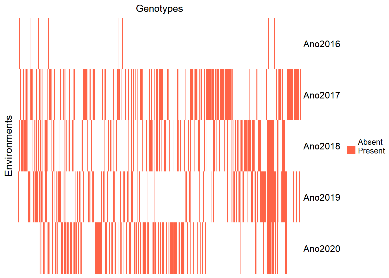
| Version | Author | Date |
|---|---|---|
| 77e21a6 | Weverton Gomes | 2025-01-13 |
Filter out the year 2016 due to insufficient observations:
Reinspect the updated heatmap:
pheno_year_count <- pheno %>%
  count(Ano, Clone)

genmat <- model.matrix(~ -1 + Clone, data = pheno_year_count)
envmat <- model.matrix(~ -1 + Ano, data = pheno_year_count)
genenvmat <- t(envmat) %*% genmat
genenvmat_ch <- ifelse(genenvmat == 1, "Present", "Absent")

Heatmap(genenvmat_ch,
        col = c("white", "tomato"),
        show_column_names = F,
        heatmap_legend_param = list(title = ""),
        column_title = "Genotypes",
        row_title = "Environments")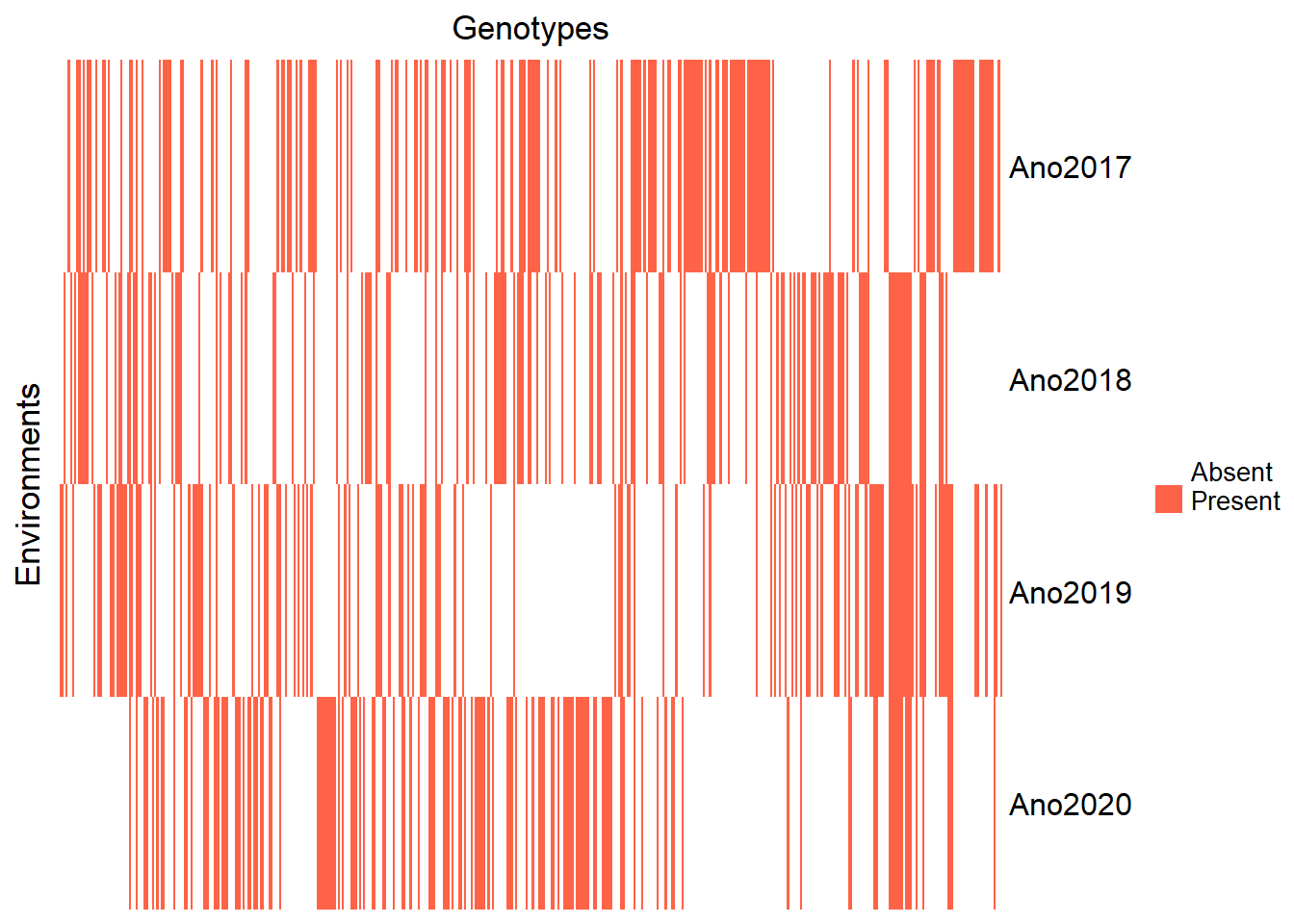
| Version | Author | Date |
|---|---|---|
| 77e21a6 | Weverton Gomes | 2025-01-13 |
Visualize the number of environments and genotypes:
genotype_year_table <- genenvmat %*% t(genenvmat) %>%
  kbl(escape = F, align = 'c') %>%
  kable_classic("hover", full_width = F, position = "center", fixed_thead = T)
rm(pheno_year_count, genmat, envmat, genenvmat, genenvmat_ch)
genotype_year_table| Ano2017 | Ano2018 | Ano2019 | Ano2020 | |
|---|---|---|---|---|
| Ano2017 | 165 | 42 | 22 | 14 |
| Ano2018 | 42 | 138 | 39 | 16 |
| Ano2019 | 22 | 39 | 133 | 29 |
| Ano2020 | 14 | 16 | 29 | 138 |
Observe that some clones were evaluated in only one year. The number of clones evaluated across different years is summarized below:
pheno %>%
  count(Ano, Clone) %>%
  count(Clone) %>%
  count(n) %>%
  kbl(escape = F, align = 'c', col.names = c("N of Environment", "N of Genotypes")) %>%
  kable_classic("hover", full_width = F, position = "center", fixed_thead = T)
Storing counts in `nn`, as `n` already present in input
ℹ Use `name = "new_name"` to pick a new name.| N of Environment | N of Genotypes |
|---|---|
| 1 | 350 |
| 2 | 72 |
| 3 | 20 |
| 4 | 5 |
Only 5 clones were evaluated in all years, which might affect the model’s accuracy. Therefore, adopting mixed models via REML in the analysis is suitable for obtaining BLUPs.
Analysis of traits
Provide descriptive statistics for each trait:
summary_table <- summary(pheno) %>%
  t() %>%
  kbl(escape = F, align = 'c') %>%
  kable_classic("hover", full_width = F, position = "center", fixed_thead = T)
summary_table| Clone | BGM-0164: 16 | BGM-0170: 16 | BGM-0396: 16 | BGM-1243: 16 | BGM-1267: 16 | BGM-0134: 12 | (Other) :2204 |
| Ano | 2017:660 | 2018:552 | 2019:532 | 2020:552 | NA | NA | NA |
| Bloco | 1:574 | 2:574 | 3:574 | 4:574 | NA | NA | NA |
| row | 11 : 121 | 3 : 120 | 10 : 120 | 2 : 119 | 6 : 118 | 4 : 117 | (Other):1581 |
| col | 6 : 131 | 4 : 130 | 8 : 130 | 2 : 128 | 5 : 128 | 9 : 128 | (Other):1521 |
| N_Roots | Min. : 0.125 | 1st Qu.: 2.333 | Median : 4.000 | Mean : 4.293 | 3rd Qu.: 6.000 | Max. :15.667 | NA’s :322 |
| FRY | Min. : 0.116 | 1st Qu.: 1.857 | Median : 3.750 | Mean : 4.946 | 3rd Qu.: 6.857 | Max. :22.200 | NA’s :335 |
| ShY | Min. : 0.694 | 1st Qu.: 6.944 | Median :11.167 | Mean :14.228 | 3rd Qu.:18.714 | Max. :61.167 | NA’s :211 |
| DMC | Min. :11.98 | 1st Qu.:25.00 | Median :28.80 | Mean :29.06 | 3rd Qu.:32.78 | Max. :48.34 | NA’s :968 |
| StY | Min. :0.0154 | 1st Qu.:0.5494 | Median :1.2068 | Mean :1.5164 | 3rd Qu.:2.1092 | Max. :8.8669 | NA’s :978 |
| Plant.Height | Min. :0.3600 | 1st Qu.:0.9633 | Median :1.1600 | Mean :1.1919 | 3rd Qu.:1.3908 | Max. :3.0333 | NA’s :220 |
| HI | Min. : 1.574 | 1st Qu.:15.726 | Median :23.345 | Mean :24.556 | 3rd Qu.:31.884 | Max. :71.967 | NA’s :341 |
| StC | Min. : 7.326 | 1st Qu.:20.350 | Median :24.147 | Mean :24.419 | 3rd Qu.:28.160 | Max. :43.686 | NA’s :968 |
| PltArc | Min. :1.000 | 1st Qu.:1.000 | Median :2.000 | Mean :1.996 | 3rd Qu.:3.000 | Max. :5.000 | NA’s :678 |
| Leaf.Ret | Min. :0.3333 | 1st Qu.:1.0000 | Median :1.3333 | Mean :1.7796 | 3rd Qu.:2.0000 | Max. :5.0000 | NA’s :216 |
| Root.Le | Min. : 7.00 | 1st Qu.:19.00 | Median :23.00 | Mean :23.21 | 3rd Qu.:27.00 | Max. :47.33 | NA’s :339 |
| Root.Di | Min. : 6.12 | 1st Qu.:23.36 | Median :28.17 | Mean :28.88 | 3rd Qu.:33.50 | Max. :63.30 | NA’s :339 |
| Stem.D | Min. :1.013 | 1st Qu.:1.859 | Median :2.101 | Mean :2.112 | 3rd Qu.:2.362 | Max. :4.373 | NA’s :224 |
| Mite | Min. :1.000 | 1st Qu.:3.000 | Median :3.667 | Mean :3.475 | 3rd Qu.:4.000 | Max. :5.000 | NA’s :222 |
| Incidence_Mites | Min. :1 | 1st Qu.:1 | Median :1 | Mean :1 | 3rd Qu.:1 | Max. :1 | NA’s :674 |
| Nstem.Plant | Min. :1.000 | 1st Qu.:1.333 | Median :2.000 | Mean :2.131 | 3rd Qu.:2.667 | Max. :6.667 | NA’s :850 |
| Stand6MAP | Min. :1.000 | 1st Qu.:4.000 | Median :6.000 | Mean :5.202 | 3rd Qu.:7.000 | Max. :8.000 | NA’s :849 |
| Branching | Min. :0.0000 | 1st Qu.:0.0000 | Median :0.3333 | Mean :0.5911 | 3rd Qu.:1.0000 | Max. :4.0000 | NA’s :673 |
| Staygreen | Min. :1.000 | 1st Qu.:1.000 | Median :1.000 | Mean :1.292 | 3rd Qu.:2.000 | Max. :3.000 | NA’s :669 |
| Vigor | Mode:logical | TRUE:1075 | NA’s:1221 | NA | NA | NA | NA |
| Flowering | Min. :0.0000 | 1st Qu.:0.0000 | Median :0.0000 | Mean :0.0074 | 3rd Qu.:0.0000 | Max. :1.0000 | NA’s :673 |
| Canopy_Lenght | Min. : 10.00 | 1st Qu.: 54.33 | Median : 72.00 | Mean : 73.35 | 3rd Qu.: 91.67 | Max. :240.17 | NA’s :1458 |
| Canopy_Width | Min. : 7.50 | 1st Qu.: 56.33 | Median : 75.58 | Mean : 76.68 | 3rd Qu.: 96.00 | Max. :213.33 | NA’s :1458 |
| Leaf_Lenght | Min. : 3.750 | 1st Qu.: 8.417 | Median :11.250 | Mean :11.676 | 3rd Qu.:14.200 | Max. :32.667 | NA’s :1459 |
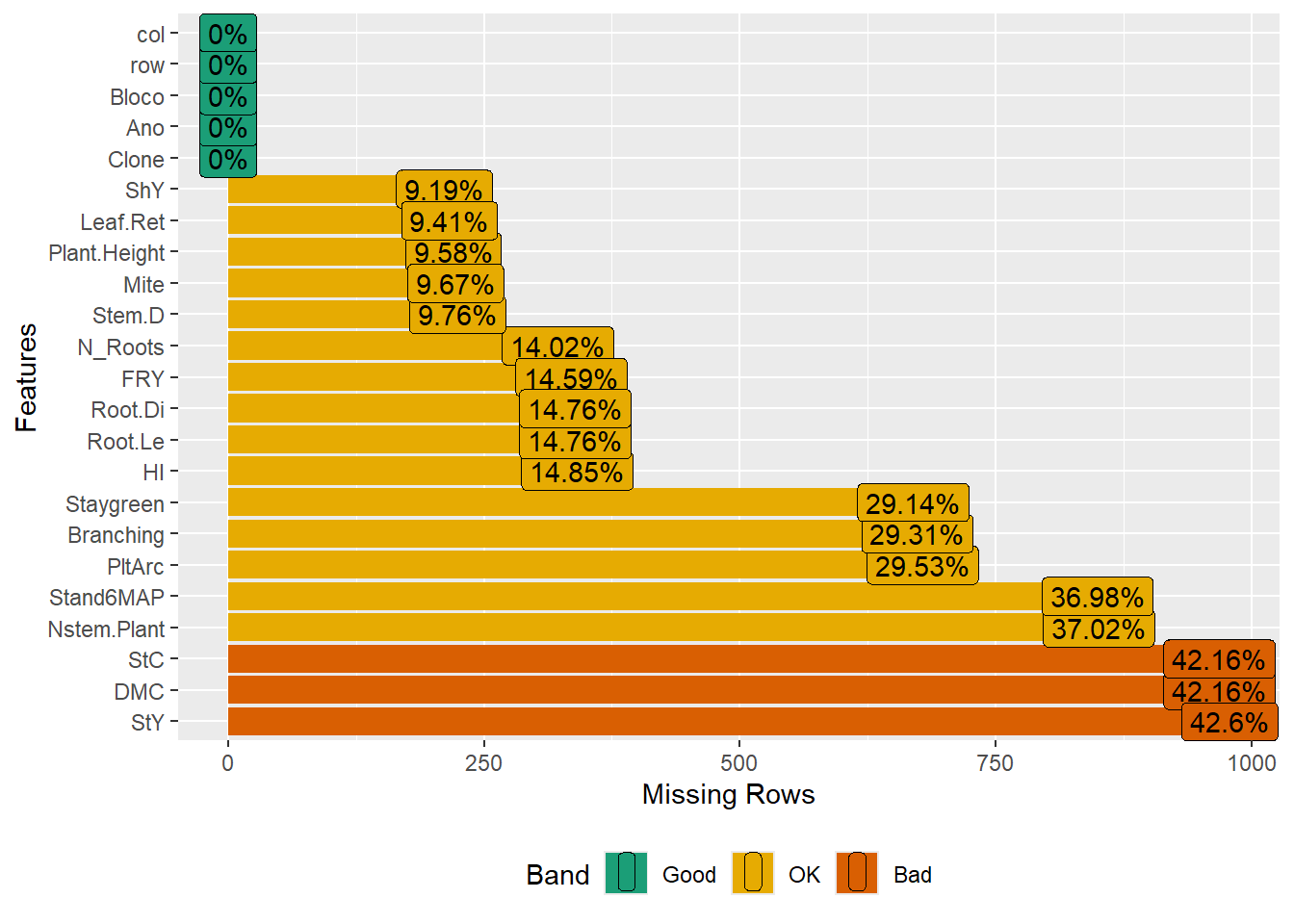
Exclude traits with high missing value ratios:
pheno <- pheno %>%
  select(-c(Incidence_Mites, Vigor, Flowering, Leaf_Lenght, Canopy_Width, Canopy_Lenght))
Ensure that the traits have acceptable missing value ratios:
| Version | Author | Date |
|---|---|---|
| 77e21a6 | Weverton Gomes | 2025-01-13 |
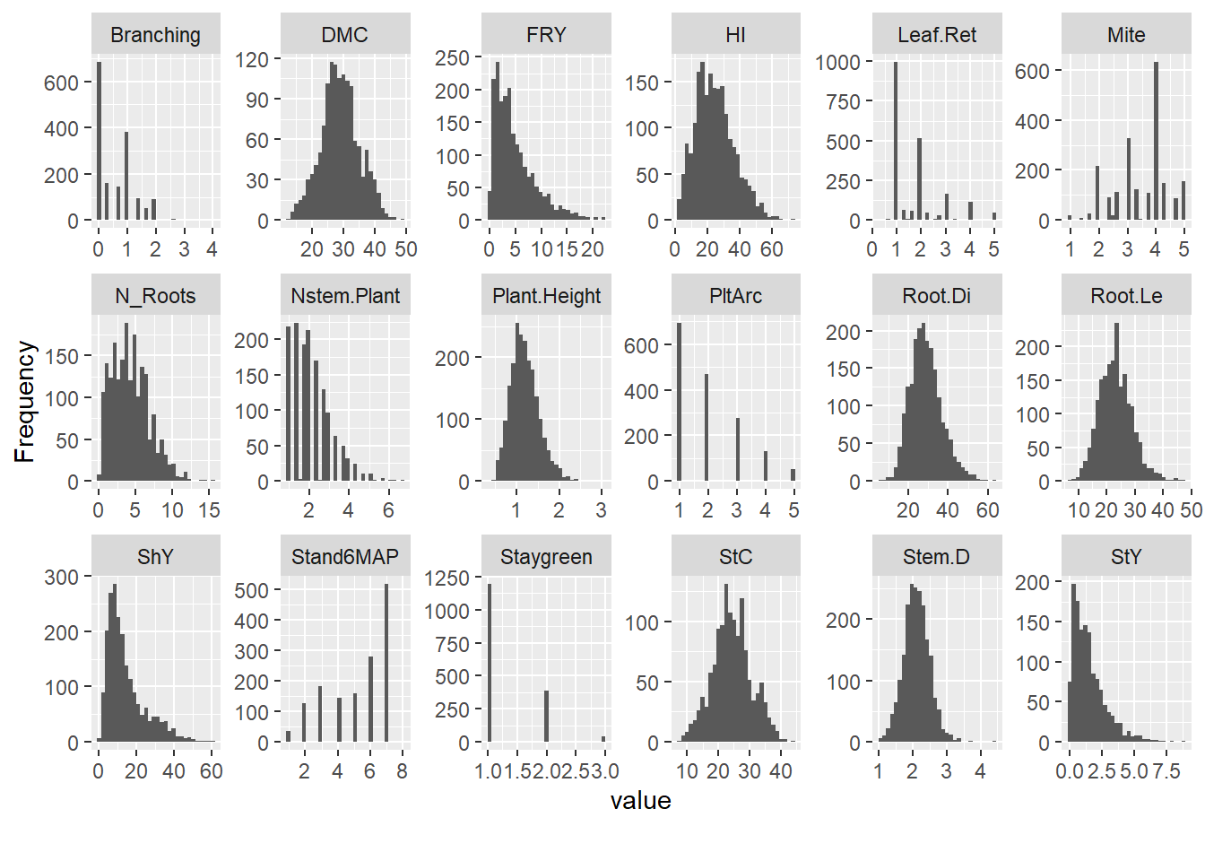
Evaluate the distribution of traits by year with histograms for quantitative traits:
| Version | Author | Date |
|---|---|---|
| 77e21a6 | Weverton Gomes | 2025-01-13 |
Remove traits that lack normal distribution:
Analisys of Clone
Inspect missing values by clone and year:
pheno_missing_summary <- pheno %>%
  select(-Bloco, -row, -col) %>%
  group_by(Clone, Ano) %>%
  summarise_all(.funs = list(~ sum(is.na(.)))) %>%
  ungroup() %>%
  select_numeric_cols() %>%
  mutate(mean = rowMeans(.),
         Clone.Ano = factor(unique(interaction(pheno$Clone, pheno$Ano)))) %>%
  filter(mean > 2) %>%
  droplevels()

missing_genotypes <- nlevels(pheno_missing_summary$Clone.Ano) %>%
  kbl(escape = F, align = 'c', col.names = c("N of genotypes")) %>%
  kable_classic("hover", full_width = F, position = "center", fixed_thead = T)
missing_genotypes| N of genotypes |
|---|
| 54 |
Evaluate clone and year descriptive statistics:
clone_year_stats <- ge_details(pheno, Ano, Clone, resp = everything()) %>%
  t() %>%
  kbl(escape = F, align = 'c') %>%
  kable_classic("hover", full_width = F, position = "center", fixed_thead = T)
clone_year_stats| Parameters | Mean | SE | SD | CV | Min | Max | MinENV | MaxENV | MinGEN | MaxGEN |
| N_Roots | 4.29 | 0.06 | 2.51 | 58.56 | 0.12 (BGM-1031 in 2017) | 15.67 (2012-107-002 in 2019) | 2018 (1.62) | 2019 (5.76) | BGM-0411 (0.33) | 2012-107-002 (11.33) |
| FRY | 4.95 | 0.09 | 4.04 | 81.79 | 0.12 (BGM-0886 in 2017) | 22.2 (BGM-1267 in 2018) | 2017 (2.75) | 2020 (6.52) | BGM-1488 (0.34) | IAC-14 (14.07) |
| ShY | 14.23 | 0.22 | 10.16 | 71.45 | 0.69 (BGM-0996 in 2017) | 61.17 (BGM-2124 in 2020) | 2017 (8.47) | 2020 (25.87) | BGM-0048 (1.52) | BGM-2124 (54.33) |
| DMC | 29.06 | 0.17 | 6.1 | 21 | 11.98 (BGM-0626 in 2020) | 48.34 (BGM-1015 in 2020) | 2020 (26.21) | 2018 (35.38) | BGM-0626 (14.98) | BGM-1015 (45.02) |
| StY | 1.52 | 0.04 | 1.27 | 84.01 | 0.02 (BGM-0340 in 2019) | 8.87 (BGM-0396 in 2018) | 2019 (1.32) | 2018 (1.84) | BGM-0089 (0.06) | BGM-1023 (4.76) |
| Plant.Height | 1.19 | 0.01 | 0.33 | 27.43 | 0.36 (BGM-0426 in 2020) | 3.03 (BR-11-24-156 in 2020) | 2017 (1) | 2019 (1.48) | Jatobá (0.58) | BGM-1200 (1.91) |
| HI | 24.56 | 0.27 | 11.89 | 48.42 | 1.57 (BGM-1159 in 2017) | 71.97 (BGM-1315 in 2018) | 2020 (18.61) | 2018 (32.36) | BGM-0961 (2.5) | Mata_Fome_Branca (52.78) |
| StC | 24.42 | 0.17 | 6.11 | 25.05 | 7.33 (BGM-0626 in 2020) | 43.69 (BGM-1015 in 2020) | 2020 (21.56) | 2018 (30.78) | BGM-0626 (10.33) | BGM-1015 (40.37) |
| Root.Le | 23.21 | 0.13 | 5.8 | 24.99 | 7 (BGM-1574 in 2017) | 47.33 (BGM-0396 in 2018) | 2017 (19.72) | 2019 (27.14) | Jatobá (8.5) | BGM-1956 (35.5) |
| Root.Di | 28.88 | 0.18 | 7.9 | 27.35 | 6.12 (BGM-2142 in 2019) | 63.3 (BRS Mulatinha in 2018) | 2017 (24.49) | 2018 (34.74) | BGM-0089 (12.14) | BGM-1956 (48.91) |
| Stem.D | 2.11 | 0.01 | 0.38 | 17.9 | 1.01 (BGM-0592 in 2018) | 4.37 (BRS Tapioqueira in 2020) | 2018 (2.02) | 2017 (2.16) | BGM-0048 (1.25) | BGM-1523 (2.93) |
| Nstem.Plant | 2.13 | 0.03 | 0.95 | 44.53 | 1 (BGM-0036 in 2018) | 6.67 (BGM-0714 in 2019) | 2018 (1.44) | 2019 (2.71) | BGM-0066 (1) | BGM-0451 (4.44) |
Again, some traits were not computed for the year 2017, so we have to eliminate that year when performing the analysis for these traits.
Evaluate the clone-only descriptive statistics for the traits.
cv_stats <- desc_stat(pheno, by = Ano, na.rm = TRUE, stats = "cv") %>%
  na.omit() %>%
  arrange(desc(cv)) %>%
  pivot_wider(names_from = "Ano", values_from = "cv") %>%
  kbl(escape = F, align = 'c') %>%
  kable_classic("hover", full_width = F, position = "center", fixed_thead = T)
cv_stats| variable | 2018 | 2020 | 2019 | 2017 |
|---|---|---|---|---|
| StY | 91.8742 | 81.2220 | 72.3243 | NA |
| FRY | 86.0073 | 68.4455 | 70.0326 | 66.8379 |
| ShY | 69.0625 | 42.7475 | 47.4901 | 45.4973 |
| N_Roots | 63.2913 | 47.0839 | 47.2357 | 48.8708 |
| HI | 41.5442 | 43.3204 | 41.8572 | 48.2942 |
| Nstem.Plant | 33.3849 | 37.1507 | 37.3740 | NA |
| Plant.Height | 28.0409 | 24.0927 | 19.1125 | 21.0398 |
| StC | 15.6937 | 27.3600 | 16.5407 | NA |
| Root.Le | 27.1625 | 18.9730 | 21.1089 | 21.5823 |
| Root.Di | 23.3943 | 20.5858 | 24.3155 | 21.0039 |
| DMC | 13.6086 | 22.5059 | 13.8212 | NA |
| Stem.D | 22.3941 | 17.5042 | 15.7037 | 16.7774 |
Some traits were not computed for the year 2017, so we have to eliminate that year when performing the analysis for these traits and some traits presented hight cv, as StY and FRY.
General Inspection
Identifying outliers in all non-categorical variables:
inspect(pheno %>%
          select_if(~ !is.factor(.)), verbose = FALSE) %>%
  arrange(desc(Outlier)) %>%
  kbl(escape = F, align = 'c') %>%
  kable_classic(
    "hover",
    full_width = F,
    position = "center",
    fixed_thead = T
)| Variable | Class | Missing | Levels | Valid_n | Min | Median | Max | Outlier | Text |
|---|---|---|---|---|---|---|---|---|---|
| ShY | numeric | Yes |
|
2085 | 0.69 | 11.17 | 61.17 | 89 | NA |
| FRY | numeric | Yes |
|
1961 | 0.12 | 3.75 | 22.20 | 71 | NA |
| StY | numeric | Yes |
|
1318 | 0.02 | 1.21 | 8.87 | 49 | NA |
| Root.Di | numeric | Yes |
|
1957 | 6.12 | 28.17 | 63.30 | 32 | NA |
| Nstem.Plant | numeric | Yes |
|
1446 | 1.00 | 2.00 | 6.67 | 30 | NA |
| Plant.Height | numeric | Yes |
|
2076 | 0.36 | 1.16 | 3.03 | 23 | NA |
| Stem.D | numeric | Yes |
|
2072 | 1.01 | 2.10 | 4.37 | 22 | NA |
| Root.Le | numeric | Yes |
|
1957 | 7.00 | 23.00 | 47.33 | 19 | NA |
| N_Roots | numeric | Yes |
|
1974 | 0.12 | 4.00 | 15.67 | 16 | NA |
| HI | numeric | Yes |
|
1955 | 1.57 | 23.35 | 71.97 | 15 | NA |
| DMC | numeric | Yes |
|
1328 | 11.98 | 28.80 | 48.34 | 6 | NA |
| StC | numeric | Yes |
|
1328 | 7.33 | 24.15 | 43.69 | 6 | NA |
Confirming what was previously described, most traits with high coefficients of variation (CV) have many outliers.
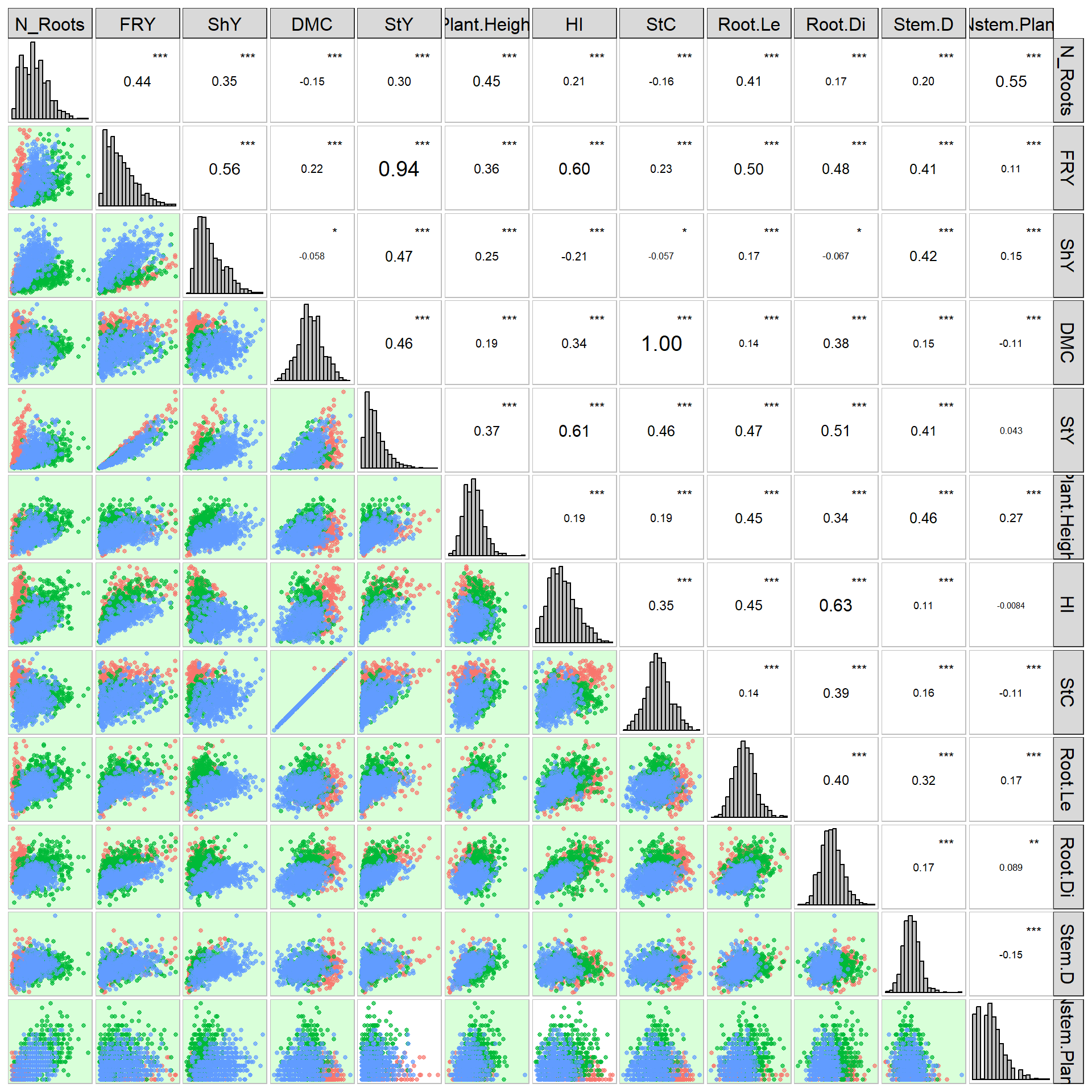
Inspect overall data correlations and save clean data:
# Descriptive statistics (mean, minimum, maximum, CV)
pheno_mean_sd <- desc_stat(pheno, stats = c("mean, min, max, cv"), na.rm = TRUE)

pheno_mean_sd %>%
  kbl(escape = F, align = 'c') %>%
kable_classic("hover", full_width = F, position = "center", fixed_thead = T)| variable | mean | min | max | cv |
|---|---|---|---|---|
| DMC | 29.0583 | 11.9760 | 48.3360 | 20.9974 |
| FRY | 4.9462 | 0.1160 | 22.2000 | 81.7937 |
| HI | 24.5559 | 1.5744 | 71.9673 | 48.4154 |
| N_Roots | 4.2929 | 0.1250 | 15.6670 | 58.5550 |
| Nstem.Plant | 2.1309 | 1.0000 | 6.6667 | 44.5279 |
| Plant.Height | 1.1919 | 0.3600 | 3.0333 | 27.4309 |
| Root.Di | 28.8785 | 6.1200 | 63.3033 | 27.3488 |
| Root.Le | 23.2147 | 7.0000 | 47.3333 | 24.9935 |
| ShY | 14.2276 | 0.6940 | 61.1670 | 71.4549 |
| StC | 24.4195 | 7.3260 | 43.6860 | 25.0456 |
| StY | 1.5164 | 0.0154 | 8.8669 | 84.0137 |
| Stem.D | 2.1125 | 1.0133 | 4.3733 | 17.8989 |
Climate data
# Load the climate data
climate_data <- read.csv("data/dados__temp_umi.csv", sep = ";", na = "null", dec = ",")

# Convert the date column to date format
climate_data$Data.Medicao <- dmy(climate_data$Data.Medicao)

# Extract the year and semester from the date
climate_data <- climate_data %>%
  mutate(Ano = year(Data.Medicao), Semestre = ifelse(month(Data.Medicao) <= 6, "1-6", "7-12"))

# Calculate the means per semester and year for each variable
semester_means <- climate_data %>%
  group_by(Ano, Semestre) %>%
  summarise_if(is.numeric, ~mean(., na.rm = TRUE))

# Display the results
semester_means %>%
  kbl(escape = F, align = 'c') %>%
kable_classic("hover", full_width = F, position = "center", fixed_thead = T)| Ano | Semestre | EVAPORACAO.DO.PICHE..DIARIA.mm. | INSOLACAO.TOTAL..DIARIO.h. | PRECIPITACAO.TOTAL..DIARIO.mm. | TEMPERATURA.MAXIMA..DIARIA..C. | TEMPERATURA.MEDIA.COMPENSADA..DIARIA..C. | TEMPERATURA.MINIMA..DIARIA..C. | UMIDADE.RELATIVA.DO.AR..MEDIA.DIARIA… | UMIDADE.RELATIVA.DO.AR..MINIMA.DIARIA… | VENTO..VELOCIDADE.MEDIA.DIARIA.m.s. |
|---|---|---|---|---|---|---|---|---|---|---|
| 2016 | 1-6 | 10.607182 | 8.453297 | 1.7829670 | 32.94780 | 27.85220 | 23.30440 | 65.63571 | 55.33516 | 2.703846 |
| 2016 | 7-12 | 13.772826 | 9.549456 | 0.1625000 | 33.72609 | 28.05217 | 22.64511 | 58.46141 | 47.90217 | 3.155978 |
| 2017 | 1-6 | 12.409945 | 8.513260 | 0.5801105 | 33.51271 | 28.48122 | 23.77845 | 60.43833 | 50.20994 | 2.971271 |
| 2017 | 7-12 | 13.032065 | 8.686957 | 0.2304348 | 32.30109 | 26.99239 | 22.08533 | 55.83770 | 44.88587 | 3.279891 |
| 2018 | 1-6 | 9.982873 | 7.917680 | 1.4602210 | 32.39779 | 27.39116 | 23.11713 | 62.37821 | 50.77348 | 2.782320 |
| 2018 | 7-12 | 12.984239 | 9.203261 | 0.3222826 | 33.13152 | 27.72283 | 22.60054 | 54.03859 | 43.55978 | 3.023913 |
| 2019 | 1-6 | 10.839326 | 8.501695 | 1.1387640 | 33.57175 | 28.31243 | 23.88596 | 61.06723 | 48.66298 | 2.758989 |
| 2019 | 7-12 | 13.895652 | 9.229891 | 0.1972826 | 33.72391 | 27.91413 | 22.59565 | 53.56667 | 43.01087 | 3.244565 |
| 2020 | 1-6 | 8.186517 | 6.869101 | 1.9252809 | 32.20337 | 27.24157 | 23.48090 | 70.01461 | 59.37234 | 2.555056 |
| 2020 | 7-12 | 12.382065 | 8.848913 | 0.9619565 | 32.79946 | 27.07017 | 21.95217 | 59.94088 | 47.12500 | 3.020109 |
Then, now we go to execute the mixed models analisys script: mixed_models.Rmd
R version 4.3.3 (2024-02-29 ucrt)
Platform: x86_64-w64-mingw32/x64 (64-bit)
Running under: Windows 10 x64 (build 19045)

Matrix products: default


locale:
[1] LC_COLLATE=Portuguese_Brazil.utf8  LC_CTYPE=Portuguese_Brazil.utf8
[3] LC_MONETARY=Portuguese_Brazil.utf8 LC_NUMERIC=C
[5] LC_TIME=Portuguese_Brazil.utf8

time zone: America/Sao_Paulo
tzcode source: internal

attached base packages:
[1] grid      stats     graphics  grDevices utils     datasets  methods
[8] base

other attached packages:
 [1] GGally_2.2.1          ggthemes_5.1.0        DataExplorer_0.8.3
 [4] metan_1.19.0          readxl_1.4.3          data.table_1.16.4
 [7] ComplexHeatmap_2.16.0 lubridate_1.9.4       forcats_1.0.0
[10] stringr_1.5.1         dplyr_1.1.4           purrr_1.0.2
[13] readr_2.1.5           tidyr_1.3.1           tibble_3.2.1
[16] ggplot2_3.5.1         tidyverse_2.0.0       kableExtra_1.4.0

loaded via a namespace (and not attached):
 [1] Rdpack_2.6.2        gridExtra_2.3       writexl_1.5.1
 [4] rlang_1.1.4         magrittr_2.0.3      clue_0.3-66
 [7] GetoptLong_1.0.5    git2r_0.35.0        matrixStats_1.5.0
[10] compiler_4.3.3      png_0.1-8           systemfonts_1.1.0
[13] vctrs_0.6.5         pkgconfig_2.0.3     shape_1.4.6.1
[16] crayon_1.5.3        fastmap_1.2.0       labeling_0.4.3
[19] promises_1.3.2      rmarkdown_2.29      tzdb_0.4.0
[22] nloptr_2.1.1        xfun_0.50           cachem_1.1.0
[25] jsonlite_1.8.9      later_1.4.1         tweenr_2.0.3
[28] parallel_4.3.3      cluster_2.1.8       R6_2.5.1
[31] bslib_0.8.0         stringi_1.8.4       RColorBrewer_1.1-3
[34] boot_1.3-31         numDeriv_2016.8-1.1 jquerylib_0.1.4
[37] cellranger_1.1.0    Rcpp_1.0.14         iterators_1.0.14
[40] knitr_1.49          IRanges_2.34.1      igraph_2.1.3
[43] httpuv_1.6.15       Matrix_1.6-1        splines_4.3.3
[46] timechange_0.3.0    tidyselect_1.2.1    rstudioapi_0.17.1
[49] yaml_2.3.10         doParallel_1.0.17   codetools_0.2-20
[52] lmerTest_3.1-3      lattice_0.22-6      plyr_1.8.9
[55] withr_3.0.2         evaluate_1.0.3      ggstats_0.8.0
[58] polyclip_1.10-7     xml2_1.3.6          circlize_0.4.16
[61] pillar_1.10.1       whisker_0.4.1       foreach_1.5.2
[64] stats4_4.3.3        reformulas_0.4.0    generics_0.1.3
[67] rprojroot_2.0.4     mathjaxr_1.6-0      S4Vectors_0.38.1
[70] hms_1.1.3           munsell_0.5.1       scales_1.3.0
[73] minqa_1.2.8         glue_1.8.0          tools_4.3.3
[76] lme4_1.1-36         fs_1.6.5            rbibutils_2.3
[79] colorspace_2.1-1    networkD3_0.4       nlme_3.1-166
[82] patchwork_1.3.0     ggforce_0.4.2       cli_3.6.3
[85] workflowr_1.7.1     viridisLite_0.4.2   svglite_2.1.3
[88] gtable_0.3.6        sass_0.4.9          digest_0.6.37
[91] BiocGenerics_0.46.0 ggrepel_0.9.6       htmlwidgets_1.6.4
[94] rjson_0.2.23        farver_2.1.2        htmltools_0.5.8.1
[97] lifecycle_1.0.4     GlobalOptions_0.1.2 MASS_7.3-60.0.1